>

plNormal

Definition 12   Given $\Omega=\{X_1,X_2,...,X_n\}$, a vector of means $\mu=(\mu_1,\mu_2,...,\mu_n)$ and an $n \times n$ variance-covariance matrix $\Sigma$. A plNormal on $\Omega$ given $\mu$ and $\Sigma$ is a kernel where the compute function is defined as follows:

$$compute(\omega) = \left\{ \begin{array}{ll} Normal(\omega,\mu,\Sigma) & \mbox{ if } \omega \in \Omega_o^\ast \\ 0 & \mbox{otherwise} \par \end{array}\right.$$ (3.5)

where

$$Normal(\omega,\mu,\Sigma) = (2\pi)^{-\frac{n}{2}}{\vert\Sigma\vert}^\frac{1}{2}\exp\left[-\frac{1}{2}(\omega-\mu)^T\Sigma^{-1}(\omega-\mu)\right]$$ (3.6)

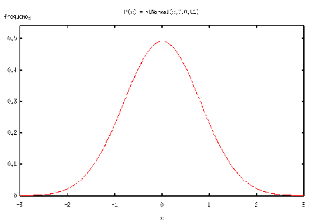
Example 4   We consider a first plNormal example for an unidimensional normal distribution. Particularly we set $\Omega =\{X\}$, $X=[-3,3]$, $\mu =0$ and $\sigma^2 = 0.81$.

図 3.4: A 1D normal kernel with $\Omega =\{X\}$, $X=[-3,3]$, $\mu =0$ and $\sigma = 0.81$.

The unidimensional plNormal kernel can be constructed by the line code below

  plNormal Px(X,0.0,0.81);

One output of the unidimensional plNormal program example shows as follows:

X = {x} with x in [-3..3]
P(x) = plNormal(x,0,0.81)

Generating 5 random values
draw # 0 = { x=0.90094 } 
draw # 1 = { x=-0.279712 } 
draw # 2 = { x=0.492526 } 
draw # 3 = { x=0.519215 } 
draw # 4 = { x=-0.576787 } 

Generating 5 best values
best # 0 = { x=0 } 
best # 1 = { x=0 } 
best # 2 = { x=0 } 
best # 3 = { x=0 } 
best # 4 = { x=0 } 

Examples of compute 
compute({ x=0 } )= 0.492521
compute({ x=-3 } )= 0.000517279
compute({ x=2.999 } )= 0.000519649
compute({ x=3 } )= 0

Observe that the value generated by best is the same at each iteration. Unlike an uniform distribution, the best value in a plNormal kernel is unique^3.1. Now observe that the function compute returns $0.0$ for { x=3 }. In effect, this value does not belongs to $\Omega_o^\ast=\{[-3.0,3.0)\}$. The resulting graph is shown by Figure 3.4.

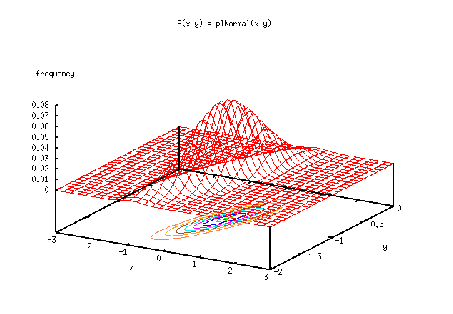
Example 5   We now show a second plNormal example for a multivariative normal kernels. Particularly we set $\Omega =\{X,Y\}$, $X=[-3,-3]$, $Y=[-2,0]$, $\mu =(0.0,-1.0)$ and

$$\Sigma = \left( \begin{array}{ll} 0.81 & 0.51 \\ 0.51 & 0.577 \end{array}\right)$$ (3.7)

図 3.5: A multivariative normal kernel with $\Omega =\{X,Y\}$, $X=[-3,-3]$, $Y=[-2,0]$, $\mu =(0.0,-1.0)$ and $\Sigma$ given by Expression (4.2).

The construction of the multivariate plNormal kernel is given by

  // Filling the parameters of the plNormal
  float matrix[4] = {0.81, 0.51,
                     0.51, 0.577};
  
  plFloatMatrix Sigma(2,matrix);
  plFloatVector mean(2);
  mean[0] = 0.0;
  mean[1] = -1.0;

  plNormal Pxy(X^Y,mean,Sigma);

One output of the multivariative plNormal shows as follow:

X = {x} with x in [-3..3]
Y = {y} with y in [-2..0]
P(x y) = plNormal(x y)

Generating 5 random values
draw # 0 = { x=1.64951 y=-0.230909 } 
draw # 1 = { x=0.916421 y=-0.145651 } 
draw # 2 = { x=-0.359675 y=-0.77395 } 
draw # 3 = { x=-0.978673 y=-1.72212 } 
draw # 4 = { x=-0.445786 y=-0.112194 } 

Generating 5 best values
best # 0 = { x=0 y=-1 } 
best # 1 = { x=0 y=-1 } 
best # 2 = { x=0 y=-1 } 
best # 3 = { x=0 y=-1 } 
best # 4 = { x=0 y=-1 } 

Examples of compute 
compute({ x=3 y=0 } )= 0
compute({ x=0 y=0 } )= 0
compute({ x=0 y=-0.0001 } )= 0.0751932
compute({ x=0 y=-1 } )= 0.29093
compute({ x=-2 y=-1 } )= 0.00615357