plGamma given
| (3.3) |
where
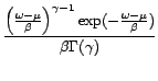 |
(3.4) |
with ![]() and
and ![]() being the gamma
function. The parameters
being the gamma
function. The parameters ![]() and
and ![]() are called the
shape, location and scale parameters respectively.
are called the
shape, location and scale parameters respectively.
plGamma kernel on
The kernel is constructed as follow
plGamma Px(X,2.0,1.0,0.0);
Here is an output example
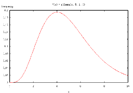
X = {x} with x in [0..10]
P(x) = plGamma(x,5,1)

Generating 5 random values
draw # 0 = { x=3.27681 }
draw # 1 = { x=3.33849 }
draw # 2 = { x=2.26463 }
draw # 3 = { x=8.31799 }
draw # 4 = { x=7.01334 }

Generating 5 best values
best # 0 = { x=4 }
best # 1 = { x=4 }
best # 2 = { x=4 }
best # 3 = { x=4 }
best # 4 = { x=4 }

Examples of compute
compute({ x=10 } )= 0.192942
compute({ x=9.99 } )= 0.194102
compute({ x=9.99 } )= 0.194102
compute({ x=9 } )= 0.344105
compute({ x=3.5 } )= 1.92581
The corresponding graph is shown by Figure 3.3.