>

Inequality constraints

An inequality constraint is used to impose one or more constraints to a set of variables $\Omega_k$. That is, to restrict the values of the variables on the set. Particularly, for $P(\Omega_s\vert\Omega_k)$ being an inequality constraint the set $\Omega_s$ is always a symbol(plSymbol) of boolean type and $\omega_s \in \Omega_s$ is true iff $\omega_k \in \Omega_k$ satisfies the constraints. In ProBT an inequality constraint is constructed by means of a function $f:\Omega_k\rightarrow I\!\!R^n$. The dimension $n$ of the resulting vector $v=(v_1,v_2,...,v_n)=f(\omega_k)$ corresponds to the number of constraints and $v_{i=1,2,...n}\leq 0$ iff the $i^{th}$ constraint is satisfied.

Definition 27   Let $\omega=(\omega_s\cup\omega_k)\in(\Omega_s\cup\Omega_k)$ with $\Omega_s$ beeing a symbol of boolean type. Given $f:\Omega_k\rightarrow I\!\!R^n$, an inequality constraint
indexconstraint on $f$ is a higher-order conditional kernel $P(\Omega_s\vert\Omega_k)$ with:

$$compute(\omega) = \left\{ \begin{array}{ll} 1 & \omega_s = f^*(\omega_k) \\ 0 & otherwise \end{array}\right.$$

and

$$instantiate(\omega_k) = dirac(\Omega_s,f^*(\omega-k) ~\mbox{ with } \omega_s = f(\omega_k)$$

with

$$f^*(\omega_k) = \left\{ \begin{array}{ll} true & \mbox{if } \forall v_i \in v=f(\omega_k): v_i\leq 0 \\ false & \mbox{otherwise} \end{array}\right.$$

Other wise stated, $compute(\omega)$ is equal to one if: (i) we ask for enforcing the constraints ($\omega_s=true$) and they are fulfilled ( $f^*(\omega_k)=true$) or (ii) if we ask for not enforcing the constraints ( $\omega_s=false$) and they are not fulfilled ( $f^*(\omega_k) =false$). Otherwise, it is equal to cero.

Example 16   Consider two variables $X,Y \in [0,10]$ having a multivariative normal kernel with $\mu=(5.0,5.0)$,

$$\Sigma = \left( \begin{array}{ll} 2.5 & 1.45 \\ 1.45 & 3.67 \end{array}\right)$$ (4.2)

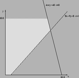
and subject to the following constraints (see Figure 4.1)

$$y+4x-40 \leq 0$$ (4.3)

$$-9y + 8x -8 \leq 0$$ (4.4)

Show the resulting kernels $P(X~Y \vert C = true)$ and $P(X~Y \vert C = false)$.

Program 13 shows a solution to our problem.

図 4.1: A constraint space with $y+4x-40 \leq 0$ and $-9y + 8x -8 \leq 0$.

Program 13: Constriants.

     1  /*=============================================================================
     2   * File           : constraint.cpp
     3   *=============================================================================
     4   *
     5   *------------------------- Description ---------------------------------------
     6   * This program shows how to impose a set of constraints to a set of variables
     7   * (use of plIneqconstraint).
     8   *-----------------------------------------------------------------------------
     9  */
    10
    11
    12  #include <pl.h>
    13
    14  /**********************************************************************
    15    Function that versifies the two imposed constraints
    16  ***********************************************************************/
    17
    18  void f_constraints(plValues &out, const plValues &in){
    19    plFloat x, y, c;
    20
    21    x = in[0];
    22    y = in[1];
    23
    24    // First constraint  y+4x-40 <= 0
    25    c = y+4*x-40;
    26    out[0] = c;
    27
    28    // Second constraint -9y + 8x -8 <= 0
    29    c = -9*y + 8*x -8;
    30    out[1] = c;
    31  }
    32
    33  main()
    34  {
    35    /**********************************************************************
    36       Defining the variable type, set and values
    37    ***********************************************************************/
    38    int i;
    39    plRealType Tx(0.0,10.0,30);
    40    plRealType Ty(0.0,10.0,30);
    41    plSymbol X("x",Tx);
    42    plSymbol Y("y",Ty);
    43    plSymbol C("c",PL_BINARY_TYPE);
    44
    45    /**********************************************************************
    46       Construction of the distribution P(X Y)
    47    ***********************************************************************/
    48
    49    // Filling the parameters of the plNormal
    50    float matrix[4] = {2.5, 1.45,
    51                       1.45, 3.67};
    52
    53    plFloatMatrix Sigma(2,matrix);
    54    plFloatVector mean(2);
    55    mean[0] = 5.0;
    56    mean[1] = 5.0;
    57
    58    // Construction of the normal kernel P(X Y)
    59    plNormal Pxy(X^Y,mean,Sigma);
    60    cout<<Pxy<<endl<<endl;
    61    plKernel Pxy_compiled;
    62
    63    // Compile and plot P(X Y | C=true)
    64    Pxy.compile(Pxy_compiled);
    65    Pxy_compiled.plot("nd_normal.gnu",30);
    66
    67    /**********************************************************************
    68      Construction of the inequality constraint P(C | X Y)
    69    ***********************************************************************/
    70    plExternalFunction ext_func(X^Y, f_constraints);
    71    plIneqConstraint Pc(C,ext_func,2);
    72
    73    /**********************************************************************
    74      Construction of the joint distribution P(X Y C) = P(X Y) P(C | X Y)
    75    ***********************************************************************/
    76
    77    // Construction of a joint distribution
    78    plJointDistribution jd(X^Y^C,Pxy^Pc);
    79    cout<<"The distribution: "<<jd<<endl;
    80
    81    /**********************************************************************
    82      Obtaining P(X Y | C = true) and P(X Y | C = false)
    83    ***********************************************************************/
    84
    85    // Geting P(X Y | C)
    86    plCndKernel Pxy_knowing_c;
    87    jd.ask(Pxy_knowing_c,X^Y,C);
    88    cout<<"Question: "<<Pxy_knowing_c<<endl;
    89
    90    // Geting P(X Y | C=true)
    91    plValues v(C);
    92    v[C] = true;
    93    plKernel Pxy_constrained;
    94    Pxy_knowing_c.instantiate(Pxy_constrained,v);
    95    cout<<"Question: "<<Pxy_constrained<<endl;
    96
    97    // Compile and plot P(X Y | C=true)
    98    Pxy_constrained.compile(Pxy_compiled);
    99    Pxy_compiled.plot("constrainted.gnu",30);
   100
   101    // Geting P(X Y | C=false)
   102    v[C] = false;
   103    plKernel Pxy_not_constrained;
   104    Pxy_knowing_c.instantiate(Pxy_not_constrained,v);
   105    cout<<"Question: "<<Pxy_not_constrained<<endl;
   106
   107    // Compile and plot P(X Y | C=false)
   108    Pxy_not_constrained.compile(Pxy_compiled);
   109    Pxy_compiled.plot("not_constrainted.gnu",30);
   110  }

The main part on the code of Program 13 is the construction of the inequality constraint $P(C \vert X Y)$ given by the following code n lines 71,72:

  plExternalFunction ext_func(X^Y, f_constraints);
  plIneqConstraint Pc(C,ext_func,2);

First, an external function is constructed with a function $f\Omega_k\rightarrow I\!\!R^n$ provided by the user. Then, the inequality constraint is constructed. The last argumet of the plIneqConstraint constructor is 2, this is because there are two constraints. The dimensionality of the output parameter out of the function f_constraints (lines 18 to 31) is then equal to this parameter. The two constraints are validated in the function provided by the user

  // First constraint  y+4x+40 <= 0
  c = y+4*x-40;
  out[0] = c;

  // Second constraint -9y + 8x -8 <= 0
  c = -9*y + 8*x -8;
  out[1] = c;

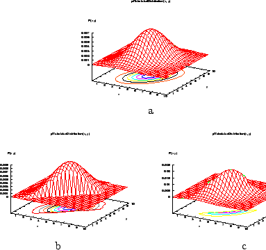
It words to say that we can stop verifying the constraints after one of them is bigger than zero. That is, the line out[0] = c; could be written as if((out[0] = c) > 0) return;. This is more efficient in terms of execution time, mainly when we have a large number of constraints to verify. Figure 4.1 shows the resulting distributions of Program 13.

図: The resulting distributions on Program 13: $P(X~Y)$ (a), $P(X~Y \vert C = true)$ (b), and $P(X~Y \vert C = false)$ (c).