plCUniform on
| (3.1) |
where
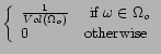 |
(3.2) |
where ![]() denotes the volume of the variable
set
denotes the volume of the variable
set ![]() .
.
Program 8 show the definition of the uniform kernel. The compute, draw and best functions are called in order to illustrate and comment their operation.
     1  /*=============================================================================
     2   * File           : uniform.cpp
     3   *=============================================================================
     4   *
     5   *------------------------- Description ---------------------------------------
     6   *This program shows the main functionalities of a continuous uniform kernel
     7   *(plCuniform).
     8   *-----------------------------------------------------------------------------
     9  */
    10
    11  #include <pl.h>
    12  #define N_TESTS 5
    13
    14  main()
    15  {
    16    /**********************************************************************
    17       Defining and printing the variable type, set and values
    18    ***********************************************************************/
    19    int i;
    20
    21    plRealType T1(0.0,10.0);
    22    plSymbol X("x",T1);
    23    plSymbol Y("y",T1);
    24    plValues Vxy(X^Y);
    25
    26    cout<<"X = "<<X<<" with x in "<<T1<<endl;
    27    cout<<"Y = "<<Y<<" with y in "<<T1<<endl;
    28
    29    /**********************************************************************
    30       Constructing, printing and ploting the kernel
    31    ***********************************************************************/
    32
    33    // Construction of the uniform kernel
    34    plCUniform Pxy(X^Y);
    35    cout<<Pxy<<endl<<endl;
    36    Pxy.plot("uniform.gnu");
    37
    38    /**********************************************************************
    39       Illustrating the main functionalities: draw, best and compute
    40    ***********************************************************************/
    41
    42    // Generating random values
    43    cout<<"Generating "<<N_TESTS<<" random values"<<endl;
    44    for(i = 0; i<N_TESTS; i++)
    45      {
    46        Pxy.draw(Vxy);
    47        cout<<"draw # "<<i<<" = "<<Vxy<<endl;
    48      }
    49
    50    // Geting the best values
    51    cout<<"\nGenerating "<<N_TESTS<<" best values"<<endl;
    52    for(i = 0; i<N_TESTS; i++)
    53      {
    54        Pxy.best(Vxy);
    55        cout<<"best # "<<i<<" = "<<Vxy<<endl;
    56      }
    57
    58    // Illustrating the compute function
    59    cout<<"\nExamples of compute \n";
    60    Vxy[X] = 10.0;  Vxy[Y] = 0.0;
    61    cout<<"compute("<<Vxy<<")= "<<Pxy.compute(Vxy)<<endl;
    62
    63    Vxy[X] = 9.99;  Vxy[Y] = 0.0;
    64    cout<<"compute("<<Vxy<<")= "<<Pxy.compute(Vxy)<<endl;
    65
    66    Vxy[X] = 9.99;  Vxy[Y] = 9.99;
    67    cout<<"compute("<<Vxy<<")= "<<Pxy.compute(Vxy)<<endl;
    68
    69    Vxy[X] = 9.0;  Vxy[Y] = 7.5;
    70    cout<<"compute("<<Vxy<<")= "<<Pxy.compute(Vxy)<<endl;
    71
    72    Vxy[X] = 3.5;  Vxy[Y] = 2.0;
    73    cout<<"compute("<<Vxy<<")= "<<Pxy.compute(Vxy)<<endl;
    74  }
An output example of Program 8 shows as as follows:
X = {x} with x in [0..10]
Y = {y} with y in [0..10]
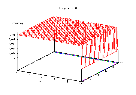
P(x y) = 0.01
Generating 5 random values
draw # 0 = { x=8.40188 y=3.94383 }
draw # 1 = { x=7.83099 y=7.9844 }
draw # 2 = { x=9.11647 y=1.97551 }
draw # 3 = { x=3.35223 y=7.6823 }
draw # 4 = { x=2.77775 y=5.5397 }
Generating 5 best values
best # 0 = { x=4.77397 y=6.28871 }
best # 1 = { x=3.64784 y=5.13401 }
best # 2 = { x=9.5223 y=9.16195 }
best # 3 = { x=6.35712 y=7.17297 }
best # 4 = { x=1.41603 y=6.06969 }
Examples of compute
compute({ x=10 y=0 } )= 0
compute({ x=9.99 y=0 } )= 0.01
compute({ x=9.99 y=9.99 } )= 0.01
compute({ x=9 y=7.5 } )= 0.01
compute({ x=3.5 y=2 } )= 0.01
Note that the set ![]() has been implicitly defined by the unique
argument of
has been implicitly defined by the unique
argument of plCUniform, line 34. In effect,
X^Y defines
![]() with
with
![]() from there
from there
![]() are implicitly constructed. Line 35 prints the
kernel. In line 36 the method
are implicitly constructed. Line 35 prints the
kernel. In line 36 the method plot generates a gnuplot file
that plots the kernel graph. For example, in this case the resulting
gnuplot file is the following:
set xlabel "x"
set ylabel "y"
set zlabel "frequency"

set xrange [0:10]
set yrange [0:10]
set zrange [0:0.011]
set nokey
set contour
set samples 200,200
set title "P(x y) =  0.01"

f(x,y)= (x>=0 & x<10 & y>=0 & y<10)? 0.01: 0
splot f(x,y)
pause -1 "Hit return to continue"
By making gnuplot uniform.gnu on a unix or linux platform you
get the graph shown at Figure 3.1. This figure
corresponds to Pxy.
Lines 42 to 48 generates random values, it worths to clarify that
all the random values are in ![]() and that no value on
and that no value on
![]() will be generated. The values
will be generated. The values
{ x=0.0 y=10.0 }, { x=10.0 y=0.0 } and
{x=10.0y=10.0 } are then impossible outputs.
The function best is called repeatedly at lines 50 to 56, note
that the obtained best values are not the same. Given that all
the elements of ![]() in a
in a plCUniform are equiprobables
the best function is equivalent to the draw function.
Finally at lines 58 to 73 we call, for different values, the compute function. Notice that, the values { x=10.0 y=0.0 }
does not belongs to ![]() by consequence the function compute returns 0.0, lines 60 and 61. In contrast, lines 63 to 73
call the compute function for values with a probability non
null.
by consequence the function compute returns 0.0, lines 60 and 61. In contrast, lines 63 to 73
call the compute function for values with a probability non
null.
In the rest of this section we illustrate examples by using the framework introduced at the beginning and exemplified by Program 8. Full programs are then not shown, just the main code lines are given. However, entire programs files can be found in the package you got with this documentation.
Our following example illustrates how to define
![]() such that it is not directly derived from
such that it is not directly derived from
![]() , that is, it is specified by the user. The specification of
, that is, it is specified by the user. The specification of
![]() requires of two more arguments on the constructor.
requires of two more arguments on the constructor.
By changing line 34 by the following code
  plFloat min[2] = {3.5,2.0};
  plFloat max[2] = {9.0,7.5};

  plCUniform Pxy(X^Y,min,max);
we get the desired plCUniform kernel.
The set ![]() is defined by two
is defined by two plFloat vectors, one for
the minimal values and the other for the maximum values. The size of
these two vectors corresponds respectively to the variables on the
first argument. That is, for X^Y the first values are
![]() and the second
and the second
![]() .
.
A run output of the new program shows as follows
X = {x} with x in [0..10]
Y = {y} with y in [0..10]
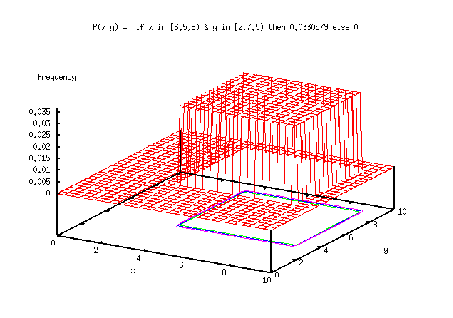
P(x y) = 0.0330579
Generating 5 random values
draw # 0 = { x=8.12103 y=4.16911 }
draw # 1 = { x=7.80705 y=6.39142 }
draw # 2 = { x=8.51406 y=3.08653 }
draw # 3 = { x=5.34373 y=6.22526 }
draw # 4 = { x=5.02776 y=5.04683 }
Generating 5 best values
best # 0 = { x=6.12568 y=5.45879 }
best # 1 = { x=5.50631 y=4.82371 }
best # 2 = { x=8.73726 y=7.03907 }
best # 3 = { x=6.99641 y=5.94513 }
best # 4 = { x=4.27881 y=5.33833 }
Examples of compute
compute({ x=10 y=0 } )= 0
compute({ x=9.99 y=0 } )= 0
compute({ x=9.99 y=9.99 } )= 0
compute({ x=9 y=7.5 } )= 0
compute({ x=3.5 y=2 } )= 0.0330579
Observe that the values generated by draw and best belongs
to ![]() and that the sub-intervals are still open at their
maximum value. Now the unique value example for which the
and that the sub-intervals are still open at their
maximum value. Now the unique value example for which the ![]() function returns a result different to 0 is
function returns a result different to 0 is { x=3.5 y=2}.
Figure 3.2 shows the corresponding graph generated by
the plot method.