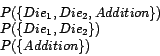
As soon as we start to think about a Bayesian modeling, we think about
all the possible outcomes of the model. For example, if we want to
observe the result of throwing two dice and the sum of them, we may
distinguish three variables: ![]() ,
, ![]() and
and ![]() . The
output of the first two variables are numbers between one and six
i.e.
. The
output of the first two variables are numbers between one and six
i.e.
![]() ; the variable
; the variable ![]() is
computed in terms of
is
computed in terms of ![]() and
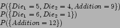
and ![]() , therefore
, therefore
![]() . For example if
. For example if ![]() and
and ![]() then
then
![]() . At this point we can make three observations:
. At this point we can make three observations:
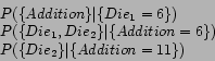
Viewed probabilistically, a variable set is an event
(e.g. ``observe the result of throwing two dice and the sum of them'') and
a variable values is and element of the event (``we
got a six in the first die, a three in the second and nine is the
sum''). Given a variable set (event) we can be interested in observing
just a subset of it. In other words, we are interested in observing
just some of the variables. Note that the observed variables
are, another event (e.g. ``observing the sum of the two
dice''). Briefly, a Bayesian model with a variable set ![]() must be capable of:
must be capable of:
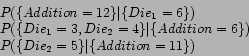
In this way variable type, sets and values are part of the essential information required to construct a Bayesian model. Any question to the model is expressed in terms of variable sets and values. In this chapter we fully describe the construction of variable types, sets and values.