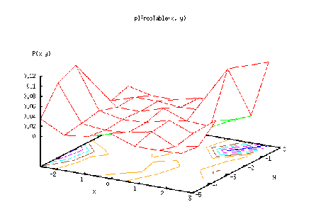
>

plProbTable

Definition 15   Let $\Omega=\{X_1,X_2,...,X_n\}$ with $Card(X_i)=m_i$ for $i=1,2,...,n$ and $A$ be an $n$ dimensional array of non negative values, where the size on dimension i is given by $m_i$. A plProbTable given $A$ is a kernel where the compute function is defined as follows:

$$Compute(\omega=\{\omega_1,\omega_2,...,\omega_n\}) = \frac{A[inde... ...dex(\omega^{\prime}_1)][index(\omega^{\prime}_2)]...[index(\omega^{\prime}_n)]}$$ (3.14)

We call $A$ the frequency distribution data.

Example 9   We show now the construction of a two-dimensional plProbTable for $\Omega=\{X_1,X_2\}$ with $X_1 = [-3.0:3.0):7$, $X_2=[-5,-4,...,0]$ and

$$A = \left( \begin{array}{rrrrrrr} 22& 56& 67& 8& 0& 7\\ 7& 10& 15& 8... ...5& 18& 6& 7& 8\\ 8& 1& 6& 4& 65& 21\\ 9& 7& 28& 18& 11& 67 \end{array}\right)$$

図 3.9: A probability table kernel.

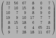The construction of the plProbTable is coded by the following lines

  plProbValue histogram[7][6] = { 22, 56, 67,  8, 0,   7,
                                   7, 10, 15,  8, 9,   0,
                                  10,  7,  9,  8, 9,   0,
                                  19,  9, 10, 17, 7,   7,
                                   8, 15, 18,  6, 7,   8,
                                   8,  1,  6,  4, 65, 21,
                                   9,  7, 28, 18, 11, 67};

  plProbTable Pxy(X^Y,*histogram);

Note that the numbers ``7'' and ``6'' on the declaration of histogram corresponds respectively to the cardinalities of $X_1$ and $X_2$ respectively. A particular point that is worth to point out is that the second argument of plProbTable must be of type plProbValue*. Consequently, if histogram were a tree-dimensional array we will pass **histogram, if it were four-dimensional, ***histogram and so on.

The output of the plProbTable kernel example is the following:

X = {x} with x in [-3 : 3)
Y = {y} with y in [-5,-4,...,0]
P(x y) =
x       y               Probability
-2.57143        -5              0.0350318
-2.57143        -4              0.089172
-2.57143        -3              0.106688
-2.57143        -2              0.0127389
-2.57143        -1              0
-2.57143        0               0.0111465
-1.71429        -5              0.0111465
-1.71429        -4              0.0159236
-1.71429        -3              0.0238854
-1.71429        -2              0.0127389
-1.71429        -1              0.0143312
-1.71429        0               0
-0.857143       -5              0.0159236
-0.857143       -4              0.0111465
-0.857143       -3              0.0143312
-0.857143       -2              0.0127389
-0.857143       -1              0.0143312
-0.857143       0               0
1.0842e-19      -5              0.0302548
1.0842e-19      -4              0.0143312
1.0842e-19      -3              0.0159236
1.0842e-19      -2              0.0270701
1.0842e-19      -1              0.0111465
1.0842e-19      0               0.0111465
0.857143        -5              0.0127389
0.857143        -4              0.0238854
0.857143        -3              0.0286624
0.857143        -2              0.00955414
0.857143        -1              0.0111465
0.857143        0               0.0127389
1.71429 -5              0.0127389
1.71429 -4              0.00159236
1.71429 -3              0.00955414
1.71429 -2              0.00636943
1.71429 -1              0.103503
1.71429 0               0.0334395
2.57143 -5              0.0143312
2.57143 -4              0.0111465
2.57143 -3              0.044586
2.57143 -2              0.0286624
2.57143 -1              0.0175159
2.57143 0               0.106688


Generating 5 random values
draw # 0 = { x=-0.614486 y=-1 }
draw # 1 = { x=2.92427 y=-4 }
draw # 2 = { x=-2.71267 y=-3 }
draw # 3 = { x=1.52381 y=0 }
draw # 4 = { x=0.837769 y=-3 }

Generating 5 best values
best # 0 = { x=2.86302 y=0 }
best # 1 = { x=2.86302 y=0 }
best # 2 = { x=2.86302 y=0 }
best # 3 = { x=2.86302 y=0 }
best # 4 = { x=2.86302 y=0 }

Examples of compute
compute({ x=3 y=0 } )= 0
compute({ x=0 y=0 } )= 0.0111465
compute({ x=0 y=0 } )= 0.0111465
compute({ x=0 y=-1 } )= 0.0111465
compute({ x=-2 y=-1 } )= 0.0143312