Bayesian Programming and Learning for Multi-Player
Video Games
Application to RTS AI
Ph.D thesis
Gabriel Synnaeve
���
Abstract
This thesis explores the use of Bayesian models in multi-player video
games AI, particularly real-time strategy (RTS) games AI. Video games are
in-between real world robotics and total simulations, as other players are not
simulated, nor do we have control over the simulation. RTS games require having
strategic (technological, economical), tactical (spatial, temporal) and reactive (units
control) actions and decisions on the go. We used Bayesian modeling as an
alternative to (boolean valued) logic, able to cope with incompleteness of
information and (thus) uncertainty. Indeed, incomplete specification of the possible
behaviors in scripting, or incomplete specification of the possible states in
planning/search raise the need to deal with uncertainty. Machine learning
helps reducing the complexity of fully specifying such models. We show that
Bayesian programming can integrate all kinds of sources of uncertainty (hidden
state, intention, stochasticity), through the realization of a fully robotic
StarCraft player. Probability distributions are a mean to convey the full
extent of the information we have and can represent by turns: constraints,
partial knowledge, state space estimation and incompleteness in the model
itself.
In the first part of this thesis, we review the current solutions to problems raised by
multi-player game AI, by outlining the types of computational and cognitive
complexities in the main gameplay types. From here, we sum up the transversal
categories of problems, introducing how Bayesian modeling can deal with all of them.
We then explain how to build a Bayesian program from domain knowledge and
observations through a toy role-playing game example. In the second part of the
thesis, we detail our application of this approach to RTS AI, and the models that we
built up. For reactive behavior (micro-management), we present a real-time
multi-agent decentralized controller inspired from sensory motor fusion. We
then show how to perform strategic and tactical adaptation to a dynamic
opponent through opponent modeling and machine learning (both supervised
and unsupervised) from highly skilled players’ traces. These probabilistic
player-based models can be applied both to the opponent for prediction, or to
ourselves for decision-making, through different inputs. Finally, we explain our
StarCraft robotic player architecture and precise some technical implementation
details.
Beyond models and their implementations, our contributions are threefolds:
machine learning based plan recognition/opponent modeling by using the structure of
the domain knowledge, multi-scale decision-making under uncertainty, and
integration of Bayesian models with a real-time control program.
Contents
Notations
Symbols
| ← | assignment of value to the left hand operand |
| ~ | the right operand is the distribution of the left operand (random variable) |
| ∝ | proportionality |
| ≈ | approximation |
| # | cardinal of a space or dimension of a variable |
| ∩ | intersection |
| ∪ | union |
| ∧ | and |
| ∨ | or |
| MT | M transposed |
| ⟦ ⟧ | integers interval |
| |
Variables
| X and V ariable | random variables (or logical propositions) |
| x and value | values |
#s =  | cardinal of the set s |
#X =  | shortcut for “cardinal of the set of the values of X” |
| X1:n | the set of n random variables X1…Xn |
| {x ∈ Ω|Q(x)} | the set of elements from Ω which verify Q |
| |
Probabilities
| P(X) = Distribution | is equivalent to X ~ Distribution |
| P(x) = P(X = x) = P([X = x]) | Probability (distribution) that X takes the value x |
| P(X,Y ) = P(X ∧ Y ) | Probability (distribution) of the conjunction of X and Y |
| P(X|Y ) | Probability (distribution) of X knowing Y |
| |
Conventions

Chapter 1
Introduction
Every game of skill is susceptible of being played by an automaton.
|
1.1 Context
1.1.1 Motivations
There is more to playing than entertainment, particularly, playing has been found to
be a basis for motor and logical learning. Real-time video games require
skill and deep reasoning, attributes respectively shared by music playing
and by board games. On many aspects, high-level real-time strategy (RTS)
players can be compared to piano players, who would write their partition
depending on how they want to play a Chess match, simultaneously to their
opponent.
Research on video games rests in between research on real-world robotics and
research on simulations or theoretical games. Indeed artificial intelligences (AI) evolve
in a simulated world that is also populated with human-controlled agents and other
AI agents on which we have no control. Moreover, the state space (set of states
that are reachable by the players) is much bigger than in board games. For
instance, the branching factor* in StarCraft is greater than 1.106, compared to
approximatively 35 in Chess and 360 in Go. Research on video games thus
constitutes a great opportunity to bridge the gap between real-world robotics and
simulations.
Another strong motivation is that there are plenty of highly skilled human video
game players, which provides inspiration and incentives to measure our artificial
intelligences against them. For RTS* games, there are professional players, whose
games are recorded. This provides datasets consisting in thousands human-hours of
play, by humans who beat any existing AI, which enables machine learning. Clearly,
there is something missing to classical AI approaches to be able to handle video
games as efficiently as humans do. I believe that RTS AI is where Chess AI was in
the early 70s: we have RTS AI world competitions but even the best entries cannot
win against skilled human players.
Complexity, real-time constraints and uncertainty are ubiquitous in video games.
Therefore video games AI research is yielding new approaches to a wide range of
problems. For instance in RTS* games: pathfinding, multiple agents coordination,
collaboration, prediction, planning and (multi-scale) reasoning under uncertainty.
The RTS framework is particularly interesting because it encompasses most of these
problems: the solutions have to deal with many objects, imperfect information,
strategic reasoning and low-level actions while running in real-time on desktop
hardware.
1.1.2 Approach
Games are beautiful mathematical problems with adversarial, concurrent and
sometimes even social dimensions, which have been formalized and studied through
game theory. On the other hand, the space complexity of video games make them
intractable problems with only theoretical tools. Also, the real-time nature of the
video games that we studied asks for efficient solutions. Finally, several video games
incorporate different forms of uncertainty, being it from partial observations or
stochasticity due to the rules. Under all these constraints, taking real-time
decisions under uncertainties and in combinatorics spaces, we have to provide a
way to program robotic video games players, whose level matches amateur
players.
We have chosen to embrace uncertainty and produce simple models which can
deal with the video games’ state spaces while running in real-time on commodity
hardware: All models are wrong; some models are useful. (attributed to Georges
Box). If our models are necessarily wrong, we have to consider that they are
approximations, and work with probabilities distributions. The other reasons to do so
confirm us in our choice:
- Partial information forces us to be able to deal with state uncertainty.
- Not only we cannot be sure about our model relevance, but how can we
assume “optimal” play from the opponent in a so complex game and so
huge state space?
The unified framework to reason under uncertainty that we used is the one of plausible
reasoning and Bayesian modeling.
As we are able to collect data about high skilled human players or produce data
through experience, we can learn the parameters of such Bayesian models. This
modeling approach unifies all the possible sources of uncertainties, learning, along
with prediction and decision-making in a consistent framework.
1.2 Contributions
We produced tractable models addressing different levels of reasoning, whose
difficulty of specification was reduced by taking advantage of machine learning
techniques, and implemented a full StarCraft AI.
- Models breaking the complexity of inference and decision in games:
- We showed that multi-agent behaviors can be authored through
inverse programming (specifying independently sensor distribution
knowing the actions), as an extension of [Hy, 2007]. We used
decentralized control (for computational efficiency) by considering
agents as sensory motor-robots: the incompleteness of not
communicating with each others is transformed into uncertainty.
- We took advantage of the hierarchy of decision-making in games
by presenting and exploiting abstractions for RTS games (strategy
& tactics) above units control. Producing abstractions, being it
through heuristics or less supervised methods, produces “bias” and
uncertainty.
- We took advantage of the sequencing and temporal continuity in
games. When taking a decision, previous observations, prediction
and decisions are compressed in distributions on variables under the
Markovian assumption.
- Machine learning on models integrating prediction and decision-making:
- We produced some of our abstractions through semi-supervised or
unsupervised learning (clustering) from datasets.
- We identified the parameters of our models from human-played
games, the same way that our models can learn from their opponents
actions / past experiences.
- An implementation of a competitive StarCraft AI able to play full games with
decent results in worldwide competitions.
Finally, video games is a billion dollars industry ($65 billion worldwide in 2011).
With this thesis, we also hope to deliver a guide for industry practitioners who would
like to have new tools for solving the ever increasing state space complexity of
(multi-scale) game AI, and produce challenging and fun to play against
AI.
1.3 Reading map
First, even though I tried to keep jargon to a minimum, when there is a precise word
for something, I tend to use it. For AI researchers, there is a lot of video games’
jargon; for game designers and programmers, there is a lot of AI jargon. I have put
everything in a comprehensive glossary.
Chapter 2 gives a basic culture about (pragmatic) game AI. The first part
explains minimax, alpha-beta and Monte-Carlo tree search by glossing over
Tic-tac-toe, Chess and Go respectively. The second part is about video games’ AI
challenges. The reader novice to AI who wants a deep introduction on artificial
intelligence can turn to the leading textbook [Russell and Norvig, 2010]. More
advanced knowledge about some specificities of game AI can be acquired by reading
the Quake III (by iD Software) source code: it is very clear and documented modern
C, and it stood the test of time in addition to being the canonical fast first person
shooter. Finally, there is no substitute for the reader novice to games to play them in
order to grasp them.
We first notice that all game AI challenge can be addressed with uncertain
reasoning, and present in chapter 3 the basics of our Bayesian modeling formalism.
As we present probabilistic modeling as an extension of logic, it may be an easy entry
to building probabilistic models for novice readers. It is not sufficient to give a strong
background on Bayesian modeling however, but there are multiple good books on the
subject. We advise the reader who want a strong intuition of Bayesian modeling to
read the seminal work by Jaynes [2003], and we found the chapter IV of the
(free) book of MacKay [2003] to be an excellent and efficient introduction
to Bayesian inference. Finally, a comprehensive review of the spectrum of
applications of Bayesian programming (until 2008) is provided by [Bessière
et al., 2008].
Chapter 4 explains the challenges of playing a real-time strategy game through
the example of StarCraft: Broodwar. It then explains our decomposition of the
problem in the hierarchical abstractions that we have studied.
Chapter 5 presents our solution to the real-time multi-agent cooperative and
adversarial problem that is micro-management. We had a decentralized reactive
behavior approach providing a framework which can be used in other games than
StarCraft. We proved that it is easy to change the behaviors by implementing several
modes with minimal code changes.
Chapter 6 deals with the tactical abstraction for partially observable games. Our
approach was to abstract low-level observations up to the tactical reasoning level
with simple heuristics, and have a Bayesian model make all the inferences at this
tactical abstracted level. The key to producing valuable tactical predictions
and decisions is to train the model on real game data passed through the
heuristics.
Chapter 7 shows our decompositions of strategy into specific prediction and
adaptation (under uncertainty) tasks. Our approach was to reduce the complexity of
strategies by using the structure of the game rules (technology trees) of expert
players vocable (openings) decisions (unit types combinations/proportions). From
partial observations, the probability distributions on the opponent’s strategy are
reconstructed, which allows for adaptation and decision-making.
Chapter 8 describes briefly the software architecture of our robotic player (bot). It
makes the link between the Bayesian models presented before and their connection
with the bot’s program. We also comment some of the bot’s debug output to show
how a game played by our bot unfolds.
We conclude by putting the contributions back in their contexts, and opening up
several perspectives for future work in the RTS AI domain.
Chapter 2
Game AI
It is not that the games and mathematical problems are chosen because
they are clear and simple; rather it is that they give us, for the smallest
initial structures, the greatest complexity, so that one can engage some
really formidable situations after a relatively minimal diversion into
programming.
Marvin Minsky (Semantic Information Processing, 1968)
|
IS the primary goal of game AI to win the game? “Game AI” is simultaneously a
research topic and an industry standard practice, for which the main metric is the
fun the players are having. Its uses range from character animation, to behavior
modeling, strategic play, and a true gameplay* component. In this chapter, we will
give our educated guess about the goals of game AI, and review what exists for a
broad category of games: abstract strategy games, partial information and/or
stochastic games, different genres of computer games. Let us then focus on gameplay
(from a player point of view) characteristics of these games so that we can enumerate
game AI needs.
2.1 Goals of game AI
2.1.1 NPC
Non-playing characters (NPC*), also called “mobs”, represent a massive volume of
game AI, as a lot of multi-player games have NPC. They really represents players
that are not conceived to be played by humans, by opposition to “bots”, which
corresponds to human-playable characters controlled by an AI. NPC are
an important part of ever more immersive single player adventures (The
Elder Scrolls V: Skyrim), of cooperative gameplays* (World of Warcraft, Left
4 Dead), or as helpers or trainers (“pets”, strategy games). NPC can be
a core part of the gameplay as in Creatures or Black and White, or dull
“quest giving poles” as in a lot of role-playing games. They are of interest for
the game industry, but also for robotics, to study human cognition and for
artificial intelligence in the large. So, the first goal of game AI is perhaps
just to make the artificial world seem alive: a paint is not much fun to play
in.
2.1.2 Win
During the last decade, the video game industry has seen the emergence of “e-sport”.
It is the professionalizing of specific competitive games at the higher levels, as in
sports: with spectators, leagues, sponsors, fans and broadcasts. A list of major
electronic sport games includes (but is not limited to): StarCraft: Brood War,
Counter-Strike, Quake III, Warcraft III, Halo, StarCraft II. The first game to have
had pro-gamers* was StarCraft: Brood War*, in Korea, with top players
earning more than Korean top soccer players. Top players earn more than
$400,000 a year but the professional average is below, around $50-60,000 a
year [Contracts, 2007], against the average South Korean salary at $16,300
in 2010. Currently, Brood War is being slowly phased out to StarCraft II.
There are TV channels broadcasting Brood War (OnGameNet, previously
also MBC Game) or StarCraft II (GOM TV, streaming) and for which it
constitutes a major chunk of the air time. “E-sport” is important to the
subject of game AI because it ensures competitiveness of the human players. It
is less challenging to write a competitive AI for game played by few and
without competitions than to write an AI for Chess, Go or StarCraft. E-sport,
through the distribution of “replays*” also ensures a constant and heavy flow
of human player data to mine and learn from. Finally, cognitive science
researchers (like the Simon Fraser University Cognitive Science Lab) study the
cognitive aspects (attention, learning) of high level RTS playing [Simon Fraser
University].
Good human players, through their ability to learn and adapt, and through
high-level strategic reasoning, are still undefeated. Single players are often frustrated
by the NPC behaviors in non-linear (not fully scripted) games. Nowadays, video
games’ AI can be used as part of the gameplay as a challenge to the player. This is
not the case in most of the games though, in decreasing order of resolution of the
problem :
fast FPS* (first person shooters), team FPS, RPG* (role playing games),
MMORPG* (Massively Multi-player Online RPG), RTS* (Real-Time Strategy).
These games in which artificial intelligences do not beat top human players on equal
footing requires increasingly more cheats to even be a challenge (not for long as
they mostly do not adapt). AI cheats encompass (but are not limited to):
- RPG NPC often have at least 10 times more hit points (health points)
than their human counterparts in equal numbers,
- FPS bots can see through walls and use perfect aiming,
- RTS bots see through the “fog of war*” and have free additional resources.
How do we build game robotic players (“bots”, AI, NPC) which can provide some
challenge, or be helpful without being frustrating, while staying fun?
2.1.3 Fun
The main purpose of gaming is entertainment. Of course, there are game genres
like serious gaming, or the “gamification*” of learning, but the majority of
people playing games are having fun. Cheating AI are not fun, and so the
replayability* of single player games is very low. The vast majority of games
which are still played after the single player mode are multi-player games,
because humans are still the most fun partners to play with. So how do
we get game AI to be fun to play with? The answer seems to be 3-fold:
- For competitive and PvP* (players versus players) games: improve game
AI so that it can play well on equal footing with humans,
- for cooperative and PvE* (players vs environment) games: optimize the
AI for fun, “epic wins”: the empowerment of playing your best and just
barely winning,
- give the AI all the tools to adapt the game to the players: AI directors*
(as in Left 4 Dead* and Dark Spore*), procedural content generation (e.g.
automatic personalized Mario [Shaker et al., 2010]).
In all cases, a good AI should be able to learn from the players’ actions, recognize their
behavior to deal with it in the most entertaining way. Examples for a few mainstream
games: World of Warcraft instances or StarCraft II missions could be less predictable
(less scripted) and always “just hard enough”, Battlefield 3 or Call of Duty opponents
could have a longer life expectancy (5 seconds in some cases), Skyrim’s follower
NPC* could avoid blocking the player in doors, or going in front when they cast
fireballs.
2.1.4 Programming
How do game developers want to deal with game AI programming? We have to
understand the needs of industry game AI programmers:
- computational efficiency: most games are real-time systems, 3D graphics
are computationally intensive, as a result the AI CPU budget is low,
- game designers often want to remain in control of the behaviors, so game
AI programmers have to provide authoring tools,
- AI code has to scale with the state spaces while being debuggable: the
complexity of navigation added to all the possible interactions with the
game world make up for an interesting “possible states coverage and
robustness” problem,
- AI behaviors have to scale with the possible game states (which are not
all predictable due to the presence of the human player),
- re-use accross games (game independant logic, at least libraries).
As a first approach, programmers can “hard code” the behaviors and their switches.
For some structuring of such states and transitions, they can and do use
state machines [Houlette and Fu, 2003]. This solution does not scale well
(exponential increase in the number of transitions), nor do they generate
autonomous behavior, and they can be cumbersome for game designers to
interact with. Hierarchical finite state machine (FSM)* is a partial answer to
these problems: they scale better due to the sharing of transitions between
macro-states and are more readable for game designers who can zoom-in on
macro/englobing states. They still represent way too much programming work for
complex behavior and are not more autonomous than classic FSM. Bakkes
et al. [2004] used an adaptive FSM mechanism inspired by evolutionary algorithms
to play Quake III team games. Planning (using a search heuristic in the
states space) efficiently gives autonomy to virtual characters. Planners like
hierarchical task networks (HTNs)* [Erol et al., 1994] or STRIPS [Fikes and
Nilsson, 1971] generate complex behaviors in the space of the combinations of
specified states, and the logic can be re-used accross games. The drawbacks
can be a large computational budget (for many agents and/or a complex
world), the difficulty to specify reactive behavior, and less (or harder) control
from the game designers. Behavior trees (Halo 2 [Isla, 2005], Spore) are a
popular in-between HTN* and hierarchical finite state machine (HFSM)*
technique providing scability through a tree-like hierarchy, control through
tree editing and some autonomy through a search heuristic. A transversal
technique for ease of use is to program game AI with a script (LUA, Python) or
domain specific language (DSL*). From a programming or design point of
view, it will have the drawbacks of the models it is based on. If everything
is allowed (low-level inputs and outputs directly in the DSL), everything
is possible at the cost of cumbersome programming, debugging and few
re-use.
Even with scalable
architectures like behavior trees or the autonomy that planning provides,
there are limitations (burdens on programmers/designers or CPU/GPU):
- complex worlds require either very long description of the state (in
propositional logic) or high expressivity (higher order logics) to specify
well-defined behaviors,
- the search space of possible actions increases exponentially with the
volume and complexity of interactions with the world, thus requiring ever
more efficient pruning techniques,
- once human players are in the loop (is it not the purpose of a game?),
uncertainty has to be taken into account. Previous approaches can be
“patched” to deal with uncertainty, but at what cost?
Our thesis is that we can learn complex behaviors from exploration or observations (of
human players) without the need to be explicitely programmed. Furthermore, the
game designers can stay in control by choosing which demonstration to learn from
and tuning parameters by hand if wanted. Le Hy et al. [2004] showed it in the case
of FPS AI (Unreal Tournament), with inverse programming to learn reactive
behaviors from human demonstration. We extend it to tactical and even strategic
behaviors.
2.2 Single-player games
Single player games are not the main focus of our thesis, but they present a few
interesting AI characteristics. They encompass all kinds of human cognitive abilities,
from reflexes to higher level thinking.
2.2.1 Action games
Platform games (Mario, Sonic), time attack racing games (TrackMania), solo
shoot-them-up (“schmups”, Space Invaders, DodonPachi), sports games and rhythm
games (Dance Dance Revolution, Guitar Hero) are games of reflexes, skill and
familiarity with the environment. The main components of game AI in these genres is
a quick path search heuristic, often with a dynamic environment. At the
Computational Intelligence and Games conferences series, there have been Mario
[Togelius et al., 2010], PacMan [Rohlfshagen and Lucas, 2011] and racing
competitions [Loiacono et al., 2008]: the winners often use (clever) heuristics coupled
with a search algorithm (A* for instance). As there are no human opponents,
reinforcement learning and genetic programming works well too. In action games, the
artificial player most often has a big advantage on its human counterpart as reaction
time is one of the key characteristics.
2.2.2 Puzzles
Point and click (Monkey Island, Kyrandia, Day of the Tentacle), graphic
adventure (Myst, Heavy Rain), (tile) puzzles (Minesweeper, Tetris) games
are games of logical thinking and puzzle solving. The main components
of game AI in these genres is an inference engine with sufficient domain
knowledge (an ontology). AI research is not particularly active in the genre of
puzzle games, perhaps because solving them has more to do with writing
down the ontology than with using new AI techniques. A classic well-studied
logic-based, combinatorial puzzle is Sudoku, which has been formulated as a
SAT-solving [Lynce and Ouaknine, 2006] and constraint satisfaction problem
[Simonis, 2005].
2.3 Abstract strategy games
2.3.1 Tic-tac-toe, minimax
Tic-tac-toe (noughts and crosses) is a solved game*, meaning that it can be played
optimally from each possible position. How did it came to get solved? Each and every
possible positions (26,830) have been analyzed by a Minimax (or its variant
Negamax) algorithm. Minimax is an algorithm which can be used to determine the
optimal score a player can get for a move in a zero-sum game*. The Minimax
theorem states:
Theorem. For every two-person, zero-sum game with finitely many strategies,
there exists a value V and a mixed strategy for each player, such that (a) Given
player 2’s strategy, the best payoff possible for player 1 is V, and (b) Given
player 1’s strategy, the best payoff possible for player 2 is -V.
Applying this theorem to Tic-tac-toe, we can say that winning is +1 point for the
player and losing is -1, while draw is 0. The exhaustive search algorithm which takes
this property into account is described in Algorithm 1. The result of applying this
algorithm to the Tic-tac-toe situation of Fig. 2.1 is exhaustively represented in
Fig. 2.2. For zero-sum games (as abstract strategy games discussed here), there is a
(simpler) Minimax variant called Negamax, shown in Algorithm 7 in Appendix A.
Algorithm 1: Minimax algorithm
function MINI(depth)
if depth ≤ 0 then
return -value()
end if
min ← +∞
for all possible moves do
score ← maxi(depth - 1)
if score < min then
min ← score
end if
end for
return min
end function
function MAXI(depth)
if depth ≤ 0 then
return value()
end if
max ←-∞
for all possible moves do
score ← mini(depth - 1)
if score > min then
max ← score
end if
end for
return max
end function
2.3.2 Checkers, alpha-beta
Checkers, Chess and Go are also zero sum, perfect-information*, partisan*,
deterministic strategy game. Theoretically, they all can be solved by exhaustive
Minimax. In practice though, it is often intractable: their bounded versions are at
least in PSPACE and their unbounded versions are EXPTIME-hard [Hearn and
Demaine, 2009]. We can see the complexity of Minimax as O(bd) with b the average
branching factor* of the tree (to search) and d the average length (depth) of the
game. For Checkers b ≈ 8, but taking pieces is mandatory, resulting in a
mean adjusted branching factor of ≈ 4, while the mean game length is 70
resulting in a game tree complexity of ≈ 1031 [Allis, 1994]. It is already too
large to have been solved by Minimax alone (on current hardware). From
1989 to 2007, there were artificial intelligence competitions on Checkers, all
using at least alpha-beta pruning: a technique to make efficient cuts in the
Minimax search tree while not losing optimality. The state space complexity of
Checkers is the smallest of the 3 above-mentioned games with ≈ 5.1020 legal
possible positions (conformations of pieces which can happen in games). As a
matter of fact, Checkers have been (weakly) solved, which means it was
solved for perfect play on both sides (and always ends in a draw) [Schaeffer
et al., 2007a]. Not all positions resulting from imperfect play have been
analyzed.
Alpha-beta pruning (see Algorithm 2) is a branch-and-bound algorithm which
can reduce Minimax search down to a O(bd∕2) = O( ) complexity if the best nodes
are searched first (O(b3d∕4) for a random ordering of nodes). α is the maximum
score that we (the maximizing player) are assured to get given what we
already evaluated, while β is the minimum score that the minimizing player is
assured to get. When evaluating more and more nodes, we can only get
a better estimate and so α can only increase while β can only decrease.
) complexity if the best nodes
are searched first (O(b3d∕4) for a random ordering of nodes). α is the maximum
score that we (the maximizing player) are assured to get given what we
already evaluated, while β is the minimum score that the minimizing player is
assured to get. When evaluating more and more nodes, we can only get
a better estimate and so α can only increase while β can only decrease.
Algorithm 2: Alpha-beta algorithm
function ALPHABETA(node,depth,α,β,player)
if depth ≤ 0 then
return value(player)
end if
if player == us then
for all possible moves do
α ← max(α,alphabeta(child,depth - 1,α,β,opponent))
if β ≤ α then
break
end if
end for
return α
else
for all possible moves do
β ← min(β,alphabeta(child,depth - 1,α,β,us))
if β ≤ α then
break
end if
end for
return β
end if
end function
If we find a node for which β becomes less than α, it means that this position
results from sub-optimal play. When it is because of an update of β, the sub-optimal
play is on the side of the maximizing player (his α is not high enough to be optimal
and/or the minimizing player has a winning move faster in the current sub-tree) and
this situation is called an α cut-off. On the contrary, when the cut results from an
update of α, it is called a β cut-off and means that the minimizing player would have
to play sub-optimally to get into this sub-tree. When starting the game, α is
initialized to -∞ and β to +∞. A worked example is given on Figure 2.3.
Alpha-beta is going to be helpful to search much deeper than Minimax in the
same allowed time. The best Checkers program (since the 90s), which is also the
project which solved Checkers [Schaeffer et al., 2007b], Chinook, has opening and
end-game (for lest than eight pieces of fewer) books, and for the mid-game (when
there are more possible moves) relies on a deep search algorithm. So, apart for
the beginning and the ending of the game, for which it plays by looking
up a database, it used a search algorithm. As Minimax and Alpha-beta
are depth first search heuristics, all programs which have to answer in a
fixed limit of time use iterative deepening. It consists in fixing limited depth
which will be considered maximal and evaluating this position. As it does not
relies in winning moves at the bottom, because the search space is too big in
branchingdepth, we need moves evaluation heuristics. We then iterate on growing
the maximal depth for which we consider moves, but we are at least sure
to have a move to play in a short time (at least the greedy depth 1 found
move).
2.3.3 Chess, heuristics
With a branching factor* of ≈ 35 and an average game length of 80 moves
[Shannon, 1950], the average game-tree complexity of chess is 3580 ≈ 3.10123.
Shannon [1950] also estimated the number of possible (legal) positions to be of the
order of 1043, which is called the Shannon number. Chess AI needed a little more
than just Alpha-beta to win against top human players (not that Checkers could not
benefit it), particularly on 1996 hardware (first win of a computer against a reigning
world champion, Deep Blue vs. Garry Kasparov). Once an AI has openings and
ending books (databases to look-up for classical moves), how can we search deeper
during the game, or how can we evaluate better a situation? In iterative deepening
Alpha-beta (or other search algorithms like Negascout [Reinefeld, 1983] or
MTD-f[Plaat, 1996]), one needs to know the value of a move at the maximal
depth. If it does not correspond to the end of the game, there is a need for an
evaluation heuristic. Some may be straight forward, like the resulting value
of an exchange in pieces points. But some strategies sacrifice a queen in
favor of a more advantageous tactical position or a checkmate, so evaluation
heuristics need to take tactical positions into account. In Deep Blue, the
evaluation function had 8000 cases, with 4000 positions in the openings
book, all learned from 700,000 grandmaster games [Campbell et al., 2002].
Nowadays, Chess programs are better than Deep Blue and generally also search
less positions. For instance, Pocket Fritz (HIARCS engine) beats current
grandmasters [Wikipedia, Center] while evaluating 20,000 positions per second (740
MIPS on a smartphone) against Deep Blue’s (11.38 GFlops) 200 millions per
second.
2.3.4 Go, Monte-Carlo tree search
With an estimated number of legal 19x19 Go positions of 2.081681994 * 10170
[Tromp and Farnebäck, 2006] (1.196% of possible positions), and an average
branching factor* above Chess for gobans* from 9x9 and above, Go sets
another limit for AI. For 19x19 gobans, the game tree complexity is up to
10360 [Allis, 1994]. The branching factor varies greatly, from ≈ 30 to 300
(361 cases at first), while the mean depth (number of plies in a game) is
between 150 to 200. Approaches other than systematic exploration of the game
tree are required. One of them is Monte Carlo Tree Search (MCTS*). Its
principle is to randomly sample which nodes to expand and which to exploit in
the search tree, instead of systematically expanding the build tree as in
Minimax. For a given node in the search tree, we note Q(node) the sum of the
simulations rewards on all the runs through node, and N(node) the visits count of
node. Algorithm 3 details the MCTS algorithm and Fig. 2.4 explains the
principle.
Algorithm 3: Monte-Carlo Tree Search algorithm. EXPANDFROM(node) is the
tree (growing) policy function on how to select where to search from situation
node (exploration or exploitation?) and how to expand the game tree (deep-first,
breadth-first, heuristics?) in case of untried actions. EVALUATE(tree) may have
2 behaviors: 1. if tree is complete (terminal), it gives an evaluation according to
games rules, 2. if tree is incomplete, it has to give an estimation, either through
simulation (for instance play at random) or an heuristic. BESTCHILD picks the
action that leads to the better value/reward from node. MERGE(node,tree)
changes the existing tree (with node) to take all the Q(ν)∀ν ∈ tree (new) values
into account. If tree contains new nodes (there were some exploration), they are
added to node at the right positions.
function MCTS(node)
while computational time left do
tree ← EXPANDFROM(node)
tree.values ← EVALUATE(tree)
MERGE(node,tree)
end while
return BESTCHILD(node)
end function
The MoGo team [Gelly and Wang, 2006, Gelly et al., 2006, 2012] introduced
the use of Upper Confidence Bounds for Trees (UCT*) for MCTS* in Go AI. MoGo
became the best 9x9 and 13x13 Go program, and the first to win against a pro on
9x9. UCT specializes MCTS in that it specifies EXPANDFROM (as in Algorithm. 4)
tree policy with a specific exploration-exploitation trade-off. UCB1 [Kocsis and
Szepesvári, 2006] views the tree policy as a multi-armed bandit problem and so
EXPANDFROM(node) UCB1 chooses the arms with the best upper confidence
bound:
 in
which k fixes the exploration-exploitation trade-off:
in
which k fixes the exploration-exploitation trade-off:  is simply the average reward
when going through c so we have exploitation only for k = 0 and exploration only for
k = ∞.
is simply the average reward
when going through c so we have exploitation only for k = 0 and exploration only for
k = ∞.
Kocsis and Szepesvári [2006] showed that the probability of selecting sub-optimal
actions converges to zero and so that UCT MCTS converges to the minimax tree and
so is optimal. Empirically, they found several convergence rates of UCT to be in
O(bd∕2), as fast as Alpha-beta tree search, and able to deal with larger problems
(with some error). For a broader survey on MCTS methods, see [Browne
et al., 2012].
With Go, we see clearly that humans do not play abstract strategy games using
the same approach. Top Go players can reason about their opponent’s move, but they
seem to be able to do it in a qualitative manner, at another scale. So, while tree
search algorithms help a lot for tactical play in Go, particularly by integrating
openings/ending knowledge, pattern macthing algorithms are not yet at the
strategical level of human players. When a MCTS algorithm learns something, it
stays at the level of possible actions (even considering positional hashing*), while the
human player seems to be able to generalize, and re-use heuristics learned at another
level.
2.4 Games with uncertainty
An exhaustive list of games, or even of games genres, is beyond the scope/range of
this thesis. All uncertainty boils down to incompleteness of information, being it
the physics of the dice being thrown or the inability to measure what is
happening in the opponent’s brain. However, we will speak of 2 types (sources) of
uncertainty: extensional uncertainty, which is due to incompleteness in direct,
measurable information, and intentional uncertainty, which is related to
randomness in the game or in (the opponent’s) decisions. Here are two extreme
illustrations of this: an agent acting without sensing is under full extensional
uncertainty, while an agent whose acts are the results of a perfect random
generator is under full intentional uncertainty. The uncertainty coming from the
opponent’s mind/cognition lies in between, depending on the simplicity to
model the game as an optimization procedure. The harder the game is to
model, the harder it is to model the trains of thoughts our opponents can
follow.
2.4.1 Monopoly
In Monopoly, there is few hidden information (Chance and Community
Chest cards only), but there is randomness in the throwing of
dice ,
and a substantial influence of the player’s knowledge of the game. A very basic
playing strategy would be to just look at the return on investment (ROI) with regard
to prices, rents and frequencies, choosing what to buy based only on the money you
have and the possible actions of buying or not. A less naive way to play should
evaluate the questions of buying with regard to what we already own, what others
own, our cash and advancement in the game. The complete state space is huge
(places for each players × their money × their possessions), but according to Ash
and Bishop [1972], we can model the game for one player (as he has no
influence on the dice rolls and decisions of others) as a Markov process on 120
ordered pairs: 40 board spaces × possible number of doubles rolled so far in
this turn (0, 1, 2). With this model, it is possible to compute more than
simple ROI and derive applicable and interesting strategies. So, even in
Monopoly, which is not lottery playing or simple dice throwing, a simple
probabilistic modeling yields a robust strategy. Additionally, Frayn [2005]
used genetic algorithms to generate the most efficient strategies for portfolio
management.
Monopoly is an example of a game in which we have complete direct information
about the state of the game. The intentional uncertainty due to the roll of the dice
(randomness) can be dealt with thanks to probabilistic modeling (Markov processes
here). The opponent’s actions are relatively easy to model due to the fact that
the goal is to maximize cash and that there are not many different efficient
strategies (not many Nash equilibrium if it were a stricter game) to attain it. In
general, the presence of chance does not invalidate previous (game theoretic /
game trees) approaches but transforms exact computational techniques into
stochastic ones: finite states machines become probabilistic Bayesian networks for
instance.
2.4.2 Battleship
Battleship (also called “naval combat”) is a guessing game generally played with two
10 × 10 grids for each players: one is the player’s ships grid, and one is to
remember/infer the opponent’s ships positions. The goal is to guess where the enemy
ships are and sink them by firing shots (torpedoes). There is incompleteness of
information but no randomness. Incompleteness can be dealt with with probabilistic
reasoning. The classic setup of the game consist in two ships of length 3 and one ship
of each lengths of 2, 4 and 5; in this setup, there are 1,925,751,392 possible
arrangements for the ships. The way to take advantage of all possible information is
to update the probability that there is a ship for all the squares each time we have
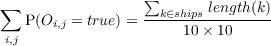
additional information. So for the 10 × 10 grid we have a 10 × 10 matrix
O1:10,1:10 with Oi,j ∈{true,false} being the ith row and jth column random
variable of the case being occupied. With ships being unsunk ships, we always
have:
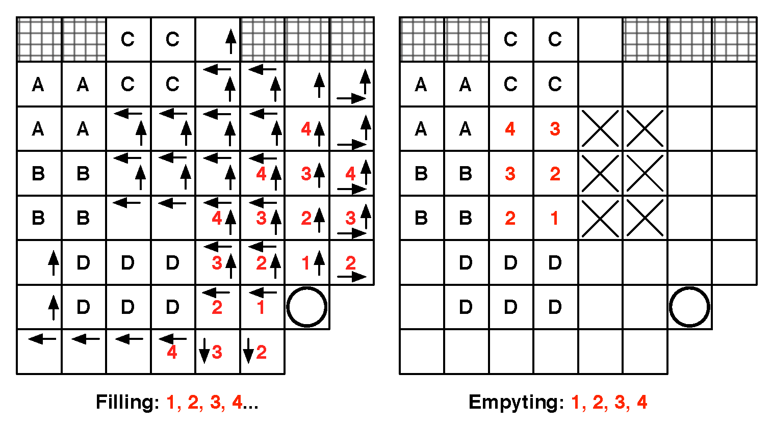
 For instance for a ship of size 3 alone at the beginning we can have prior
distributions on O1:10,1:10 by looking at combinations of its placements (see
Fig. 2.5). We can also have priors on where the opponent likes to place her
ships. Then, in each round, we will either hit or miss in i,j. When we hit,
we know P(Oi,j = true) = 1.0 and will have to revise the probabilities of
surrounding areas, and everywhere if we learned the size of the ship, with possible
placement of ships. If we did not sunk a ship, the probabilities of uncertain (not
0.0 or 1.0) positions around i,j will be highered according to the sizes of
remaining ships. If we miss, we know P([Oi,j = false]) = 1.0 and can also revise
(lower) the surrounding probabilities, an example of that effect is shown in
Fig. 2.5.
For instance for a ship of size 3 alone at the beginning we can have prior
distributions on O1:10,1:10 by looking at combinations of its placements (see
Fig. 2.5). We can also have priors on where the opponent likes to place her
ships. Then, in each round, we will either hit or miss in i,j. When we hit,
we know P(Oi,j = true) = 1.0 and will have to revise the probabilities of
surrounding areas, and everywhere if we learned the size of the ship, with possible
placement of ships. If we did not sunk a ship, the probabilities of uncertain (not
0.0 or 1.0) positions around i,j will be highered according to the sizes of
remaining ships. If we miss, we know P([Oi,j = false]) = 1.0 and can also revise
(lower) the surrounding probabilities, an example of that effect is shown in
Fig. 2.5.
Battleship is a game with few intensional uncertainty (no randomness),
particularly because the goal quite strongly conditions the action (sink ships as fast
as possible). However, it has a large part of extensional uncertainty (incompleteness
of direct information). This incompleteness of information goes down rather quickly
once we act, particularly if we update a probabilistic model of the map/grid. If we
compare Battleship to a variant in which we could see the adversary board, playing
would be straightforward (just hit ships we know the position on the board), now in
real Battleship we have to model our uncertainty due to the incompleteness of
information, without even beginning to take into account the psychology
of the opponent in placement as a prior. The cost of solving an imperfect
information game increases greatly from its perfect information variant: it seems to
be easier to model stochasticity (or chance, a source of randomness) than
to model a hidden (complex) system for which we only observe (indirect)
effects.
2.4.3 Poker
Poker
is a zero-sum (without the house’s cut), imperfect information and stochastic
betting game. Poker “AI” is as old as game theory [Nash, 1951], but the
research effort for human-level Poker AI started in the end of the 90s. The
interest for Poker AI is such that there are annual AAAI computer Poker
competitions .
Billings et al. [1998] defend Poker as an interesting game for decision-making
research, because the task of building a good/high level Poker AI (player) entails to
take decisions with incomplete information about the state of the game, incomplete
information about the opponents’ intentions, and model their thoughts process to be
able to bluff efficiently. A Bayesian network can combine these uncertainties and
represent the player’s hand, the opponents’ hands and their playing behavior
conditioned upon the hand, as in [Korb et al., 1999]. A simple “risk evaluating” AI
(folding and raising according to the outcomes of its hands) will not prevail
against good human players. Bluffing, as described by Von Neumann and
Morgenstern [1944] “to create uncertainty in the opponent’s mind”, is an element of
Poker which needs its own modeling. Southey et al. [2005] also give a Bayesian
treatment to Poker, separating the uncertainty resulting from the game (draw of
cards) and from the opponents’ strategies, and focusing on bluff. From a
game theoretic point of view, Poker is a Bayesian game*. In a Bayesian
game, the normal form representation requires describing the strategy spaces,
type spaces, payoff and belief functions for each player. It maps to all the
possible game trees along with the agents’ information state representing
the probabilities of individual moves, called the extensive form. Both these
forms scale very poorly (exponentially). Koller and Pfeffer [1997] used the
sequence form transformation, the set of realization weights of the sequences of
moves ,
to search over the space of randomized strategies for Bayesian games automatically.
Unfortunately, strict game theoretic optimal strategies for full-scale Poker are still
not tractable this way, two players Texas Hold’em having a state space ≈ O(1018).
Billings et al. [2003] approximated the game-theoretic optimal strategies
through abstraction and are able to beat strong human players (not world-class
opponents).
Poker is a game with both extensional and intentional uncertainty, from the fact
that the opponents’ hands are hidden, the chance in the draw of the cards, the
opponents’ model about the game state and their model about our mental state(s)
(leading our decision(s)). While the iterated reasoning (“if she does A, I
can do B”) is (theoretically) finite in Chess due to perfect information, it is
not the case in Poker (“I think she thinks I think...”). The combination of
different sources of uncertainty (as in Poker) makes it complex to deal with it
(somehow, the sources of uncertainty must be separated), and we will see
that both these sources of uncertainties arise (at different levels) in video
games.
2.5 FPS
2.5.1 Gameplay and AI
First person shooters gameplay* consist in controlling an agent in first person
view, centered on the weapon, a gun for instance. The firsts FPS popular
enough to bring the genre its name were Wolfeinstein 3D and Doom, by iD
Software. Other classic FPS (series) include Duke Nukem 3D, Quake, Half-Life,
Team Fortress, Counter-Strike, Unreal Tournament, Tribes, Halo, Medal of
Honor, Call of Duty, Battlefield, etc. The distinction between “fast FPS”
(e.g. Quake series, Unreal Tournament series) and others is made on the
speed at which the player moves. In “fast FPS”, the player is always jumping,
running much faster and playing more in 3 dimensions than on discretely
separate 2D ground planes. Game types include (but are not limited to):
- single-player missions, depending of the game design.
- capture-the-flag (CTF), in which a player has to take the flag inside the
enemy camp and bring it back in her own base.
- free-for-all (FFA), in which there are no alliances.
- team deathmatch (TD), in which two (or more) teams fight on score.
- various gather and escort (including hostage or payload modes), in which
one team has to find and escort something/somebody to another location.
- duel/tournament/deathmatch, 1 vs 1 matches (mainly “fast FPS”).
From these various game types, the player has to maximize its damage (or positive
actions) output while staying alive. For that, she will navigate her avatar in an
uncertain environment (partial information and other players intentions) and shoot
(or not) at targets with specific weapons.
Some games allow for instant (or delayed, but asynchronous to other players)
respawn (recreation/rebirth of a player), most likely in the “fast FPS” (Quake-like)
games, while in others, the player has to wait for the end of the round to respawn. In
some games, weapons, ammunitions, health, armor and items can be picked on the
ground (mainly “fast FPS”), in others, they are fixed at the start or can be
bought in game (with points). The map design can make the gameplay vary
a lot, between indoors, outdoors, arena-like or linear maps. According to
maps and gameplay styles, combat may be well-prepared with ambushes,
sniping, indirect (zone damages), or close proximity (even to fist weapons).
Most often, there are strong tactical positions and effective ways to attack
them.
While “skill” (speed of the movements, accuracy of the shots) is easy to emulate
for an AI, team-play is much harder for bots and it is always a key ability. Team-play
is the combination of distributed evaluation of the situation, planning and
distribution of specialized tasks. Very high skill also requires integrating over enemy’s
tactical plans and positions to be able to take indirect shots (grenades for instance)
or better positioning (coming from their back), which is hard for AI too. An example
of that is that very good human players consistently beat the best bots (nearing
100% accuracy) in Quake III (which is an almost pure skill “fast FPS”), because they
take advantage of being seen just when their weapons reload or come from
their back. Finally, bots which equal the humans by a higher accuracy are
less fun to play with: it is a frustrating experience to be shot across the
map, by a bot which was stuck in the door because it was pushed out of its
trail.
2.5.2 State of the art
FPS AI consists in controlling an agent in a complex world: it can have to
walk, run, crouch, jump, swim, interact with the environment and tools, and
sometimes even fly. Additionally, it has to shoot at moving, coordinated and
dangerous, targets. On a higher level, it may have to gather weapons, items or
power-ups (health, armor, etc.), find interesting tactical locations, attack, chase,
retreat...
The Quake III AI is a standard for Quake-like games [van Waveren and
Rothkrantz, 2002]. It consists in a layered architecture (hierarchical) FSM*. At the
sensory-motor level, it has an Area Awareness System (AAS) which detects collisions,
accessibility and computes paths. The level above provides intelligence for chat,
goals (locations to go to), and weapons selection through fuzzy logic. Higher
up, there are the behavior FSM (“seek goals”, chase, retreat, fight, stand...)
and production rules (if-then-else) for squad/team AI and orders. A team
of bots always behaves following the orders of one of the bots. Bots have
different natures and tempers, which can be accessed/felt by human players,
specified by fuzzy relations on “how much the bot wants to do, have, or
use something”. A genetic algorithm was used to optimize the fuzzy logic
parameters for specific purposes (like performance). This bot is fun to play
against and is considered a success, however Quake-like games makes it easy
to have high level bots because very good players have high accuracy (no
fire spreading), so they do not feel cheated if bots have a high accuracy
too. Also, the game is mainly indoors, which facilitates tactics and terrain
reasoning. Finally, cooperative behaviors are not very evolved and consist
in acting together towards a goal, not with specialized behaviors for each
agent.
More recent FPS games have dealt with these limitations by using combinations
of STRIPS planning (F.E.A.R. [Orkin, 2006]), HTN* (Killzone 2 [Champandard
et al., 2009] and ArmA [van der Sterren, 2009]), Behavior trees (Halo 2
[Isla, 2005]). Left4Dead (a cooperative PvE FPS) uses a global supervisor of the
AI to set the pace of the threat to be the most enjoyable for the player
[Booth, 2009].
In research, Laird [2001] focused on learning rules for opponent modeling,
planning and reactive planning (on Quake), so that the robot builds plan by
anticipating the opponent’s actions. Le Hy et al. [2004], Hy [2007] used
robotics inspired Bayesian models to quickly learn the parameters from human
players (on Unreal Tournament). Zanetti and Rhalibi [2004] and Westra and
Dignum [2009] applied evolutionary neural networks to optimize Quake
III bots. Predicting opponents positions is a central task to believability
and has been solved successfully using particle filters [Bererton, 2004] and
other models (like Hidden Semi-Markov Models) [Hladky and Bulitko, 2008].
Multi-objective neuro-evolution [Zanetti and Rhalibi, 2004, Schrum et al., 2011]
combines learning from human traces with evolutionary learning for the
structure of the artificial neural network, and leads to realistic (human-like)
behaviors, in the context of the BotPrize challenge (judged by humans)
[Hingston, 2009].
2.5.3 Challenges
Single-player FPS campaigns immersion could benefit from more realistic bots and
clever squad tactics. Multi-player FPS are competitive games, and a better game AI
should focus on:
- believability requires the AI to take decisions with the same informations
than the human player (fairness) and to be able to deal with unknown
situation.
- surprise and unpredictability is key for both performance and the
long-term interest in the human player in the AI.
- performance, to give a challenge to human players, can be achieved
through cooperative, planned and specialized behaviors.
2.6 (MMO)RPG
2.6.1 Gameplay and AI
Inspired directly by tabletop and live action role-playing games (Dungeon &
Dragons) as new tools for the game masters, it is quite natural for the RPG to have
ended up on computers. The firsts digital RPG were text (Wumpus) or
ASCII-art (Rogue, NetHack) based. The gameplay evolved considerably
with the technique. Nowadays, what we will call a role playing game (RPG)
consist in the incarnation by the human player of an avatar (or a team of
avatars) with a class: warrior, wizard, rogue, priest, etc., having different skills,
spells, items, health points, stamina/energy/mana (magic energy) points.
Generally, the story brings the player to solve puzzles and fight. In a fight,
the player has to take decisions about what to do, but skill plays a lesser
role in performing the action than in a FPS game. In a FPS, she has to
move the character (egocentrically) and aim to shoot; in a RPG, she has
to position itself (often way less precisely and continually) and just decide
which ability to use on which target (or a little more for “action RPG”). The
broad category of RPG include: Fallout, The Elders Scrolls (from Arena
to Skyrim), Secret of Mana, Zelda, Final Fantasy, Diablo, Baldur’s Gate.
A MMORPG (e.g. World of Warcraft, AION or EVE Online) consist in
a role-playing game in a persistent, multi-player world. There usually are
players-run factions fighting each others’ (PvP) and players versus environment
(PvE) situations. PvE* may be a cooperative task in which human players
fight together against different NPC, and in which the cooperation is at the
center of the gameplay. PvP is also a cooperative task, but more policy and
reactions-based than a trained and learned choregraphy as for PvE. We can
distinguish three types (or modality) of NPC which have different game AI needs:
- world/neutral/civilian NPC: gives quests, takes part in the world’s or
game’s story, talks,
- “mob”/hostile NPC that the player will fight,
- “pets”/allied NPC: acts by the players’ sides.
- persistent character AI could maintain the players’ avatars in the world
when they are disconnected.
NPC acting strangely are sometimes worse for the player’s immersion than immobile and
dull ones. However, it is more fun for the player to battle with hostile NPC which are
not too dumb or predictable. Players really expect allied NPC to at least not
hinder them, and it is even better when they adapt to what the player is
doing.
2.6.2 State of the art
Methods used in FPS* are also used in RPG*. The needs are sometimes a little
different for RPG games: for instance RPG need interruptible behaviors, behaviors
that can be stopped and resumed (dialogs, quests, fights...) that is. RPG also require
stronger story-telling capabilities than other gameplay genres, for which they use
(logical) story representations (ontologies) [Kline, 2009, Riedl et al., 2011].
Behavior multi-queues [Cutumisu and Szafron, 2009] resolve the problems of having
resumable, collaborative, real-time and parallel behavior, and tested their approach
on Neverwinter Nights. Basically they use prioritized behavior queues which can be
inserted (for interruption and resumption) in each others. AI directors are control
programs tuning the difficulty and pace of the game session in real-time from
player’s metrics. Kline [2011] used an AI director to adapt the difficulty of
Dark Spore to the performance (interactions and score) of the player in
real-time.
2.6.3 Challenges
There are mainly two axes for RPG games to bring more fun: interest in the game
play(s), and immersion. For both these topics, we think game AI can bring a lot:
- believability of the agents will come from AI approaches than can deal
with new situations, being it because they were not dealt with during
game development (because the “possible situations” space is too big) or
because they were brought by the players’ unforeseeable actions. Scripts
and strict policies approaches will be in difficulty here.
- interest (as opposed to boredom) for the human players in the game style
of the AI will come from approaches which can generate different behaviors
in a given situation. Expectable AI particularly affects replayability
negatively.
- performance relative to the gameplay will come from AI approaches
than can fully deal with cooperative behavior. One solution is to design
mobs to be orders of magnitude stronger (in term of hit points and
damages) than players’ characters, or more numerous. Another, arguably
more entertaining, solution is to bring the mobs behavior to a point where
they are a challenge for the team of human players.
Both believability and performance require to deal with uncertainty of the game
environment. RPG AI problem spaces are not tractable for a frontal (low-level)
search approach nor are there few enough situations to consider to just write a bunch
of script and puppeteer artificial agents at any time.
2.7 RTS Games
As RTS are the central focus on this thesis, we will discuss specific problems and
solution more in depth in their dedicated chapters, simply brushing here the
underlying major research problems. Major RTS include the Command&Conquer,
Warcraft, StarCraft, Age of Empires and Total Annihilation series.
2.7.1 Gameplay and AI
RTS gameplay consist in gathering resources, building up an economic and military
power through growth and technology, to defeat your opponent by destroying his
base, army and economy. It requires dealing with strategy, tactics, and units
management (often called micro-management) in real-time. Strategy consist in
what will be done in the long term as well as predicting what the enemy is
doing. It particularly deals with the economy/army trade-off estimation, army
composition, long-term planning. The three aggregate indicators for strategy are
aggression, production, and technology. The tactical aspect of the gameplay is
dominated by military moves: when, where (with regard to topography and weak
points), how to attack or defend. This implies dealing with extensional (what
the invisible units under “fog of war*” are doing) and intentional (what
will the visible enemy units do) uncertainty. Finally, at the actions/motor
level, micro-management is the art of maximizing the effectiveness of the
units i.e. the damages given/damages received ratio. For instance: retreat
and save a wounded unit so that the enemy units would have to chase it
either boosts your firepower or weakens the opponent’s. Both [Laird and van
Lent, 2001] and Gunn et al. [2009] propose that RTS AI is one of the most
challenging genres, because all levels in the hierarchy of decisions are of
importance.
More will be said about RTS in the dedicated chapter 4.
2.7.2 State of the art & challenges
Buro [2004] called for AI research in RTS games and identified the technical
challenges as:
- adversarial planning under uncertainty, and for that abstractions
have to be found both allowing to deal with partial observations and to
plan in real-time.
- learning and opponent modeling: adaptability plays a key role in the
strength of human players.
- spatial and temporal reasoning: tactics using the terrain features and
good timings are essential for higher level play.
To these challenges, we would like to add the difficulty of inter-connecting all special
cases resolutions of these problems: both for the collaborative (economical and
logistical) management of the resources, and for the sharing of uncertainty
quantization in the decision-making processes. Collaborative management of the
resources require arbitrage between sub-models on resources repartition. By sharing
information (and its uncertainty) between sub-models, decisions can be made
that account better for the whole knowledge of the AI system. This will be
extended further in the next chapters as RTS are the main focus of this
thesis.
2.8 Games characteristics
All the types of video games that we saw before require to deal with imperfect
information and sometimes with randomness, while elaborating a strategy (possibly
from underlying policies). From a game theoretic point of view, these video games are
close to what is called a Bayesian game* [Osborne and Rubinstein, 1994].
However, solving Bayesian games is non-trivial, there are no generic and
efficient approaches, and so it has not been done formally for card games with
more than a few cards. Billings et al. [2003] approximated a game theoretic
solution for Poker through abstraction heuristics, it leads to believe than game
theory can be applied at the higher (strategic) abstracted levels of video
games.
We do not pretend to do a complete taxonomy of video games and AI (e.g. [Gunn
et al., 2009]), but we wish to provide all the major informations to differentiate
game genres (gameplays). To grasp the challenges they pose, we will provide abstract
measures of complexity.
2.8.1 Combinatorics
“How does the state of possible actions grow?” To measure this, we used a measure
from perfect information zero-sum games (as Checkers, Chess and Go): the branching
factor* b and the depth d of a typical game. The complexity of a game (for taking a
decision) is proportional to bd. The average branching factor for a board game is easy
to compute: it is the average number of possible moves for a given player. For Poker,
we set b = 3 for fold, check and raise. d should then be defined over some time, the
average number of events (decisions) per hour in Poker is between 20 to 240. For
video-games, we defined b to be the average number of possible moves at
each decision, so for “continuous” or “real-time” games it is some kind of
function of the useful discretization of the virtual world at hand. d has to
be defined as a frequency at which a player (artificial or not) has to take
decisions to be competitive in the game, so we will give it in d∕time_unit.
For instance, for a car (plane) racing game, b ≈ 50 - 500 because b is a
combination of throttle (ẍ) and direction (θ) sampled values that are relevant
for the game world, with d∕min at least 60: a player needs to correct her
trajectory at least once a second. In RTS games, b ≈ 200 is a lower bound
(in StarCraft we may have between 50 to 400 units to control), and very
good amateurs and professional players perform more than 300 actions per
minute.
The sheer size of b and d in video games make it seem intractable, but
humans are able to play, and to play well. To explain this phenomenon,
we introduce “vertical” and “horizontal” continuities in decision making.
Fig. 2.6 shows how one can view the decision-making process in a video
game: at different time scales, the player has to choose between strategies to
follow, that can be realized with the help of different tactics. Finally, at
the action/output/motor level, these tactics have to be implemented one
way or another. So, matching Fig. 2.6, we could design a Bayesian model:
- St,t-1 ∈ Attack,Defend,Collect,Hide, the strategy variable
- Tt,t-1 ∈ Front,Back,Hit - and - run,Infiltrate, the tactics variable
- At,t-1 ∈ low_level_actions, the actions variable
- O1:nt ∈{observations}, the set of observations variables


- P(St|St-1,O1:nt) should be read as “the probability distribution on the
strategies at time t is determined/influenced by the strategy at time t- 1
and the observations at time t”.
- P(Tt|St,Tt-1,O1:nt) should be read as “the probability distribution on
the tactics at time t is determined by the strategy at time t, tactics at
time t - 1 and the observations at time t”.
- P(At|Tt,At-1,O1:nt) should be read as “the probability distribution on
the actions at time t is determined by tactics at time t, the actions at time
t - 1 and the observations at time t”.
Vertical continuity
In the decision-making process, vertical continuity describes when taking a
higher-level decision implies a strong conditioning on lower-levels decisions. As seen
on Figure 2.7: higher level abstractions have a strong conditioning on lower levels.
For instance, and in non-probabilistic terms, if the choice of a strategy s (in the
domain of S) entails a strong reduction in the size of the domain of T, we consider
that there is a vertical continuity between S and T. There is vertical continuity
between S and T if ∀s ∈{S},{P(Tt|[St = s],Tt-1,O1:nt) > ϵ} is sparse in
{P(Tt|Tt-1,O1:nt) > ϵ}. There can be local vertical continuity, for which the
previous statement holds only for one (or a few) s ∈{S}, which are harder to
exploit. Recognizing vertical continuity allows us to explore the state space
efficiently, filtering out absurd considerations with regard to the higher decision
level(s).
Horizontal continuity
Horizontal continuity also helps out cutting the search in the state space to only
relevant states. At a given abstraction level, it describes when taking a decision
implies a strong conditioning on the next time-step decision (for this given level). As
seen on Figure 2.8: previous decisions on a given level have a strong conditioning on
the next ones. For instance, and in non-probabilistic terms, if the choice of a tactic t
(in the domain of Tt) entails a strong reduction in the size of the domain of Tt+1, we
consider that T has horizontal continuity. There is horizontal continuity
between Tt-1 and Tt if ∀t ∈{T},{P(Tt|St,[Tt-1 = t],O1:nt) > ϵ} is sparse in
{P(Tt|St,O1:nt) > ϵ}. There can be local horizontal continuity, for which the
previous state holds only for one (or a few) t ∈{T}. Recognizing horizontal
continuity boils down to recognizing sequences of (frequent) actions from
decisions/actions dynamics and use that to reduce the search space of subsequent
decisions. Of course, at a sufficiently small time-step, most continuous games have
high horizontal continuity: the size of the time-step is strongly related to the design
of the abstraction levels for vertical continuity.
2.8.2 Randomness
Randomness can be inherent to the gameplay. In board games and table top
role-playing, randomness often comes from throwing dice(s) to decide the outcome of
actions. In decision-making theory, this induced stochasticity is dealt with in the
framework of a Markov decision process (MDP)*. A MDP is a tuple of (S,A,T,R)
with:
- S a finite set of states
- A a finite set of actions
- Ta(s,s′) = P([St+1 = s′]|[St = s],[At = a]) the probability that action a
in state s at time t will lead to state s′ at time t + 1
- Ra(s,s′) the immediate reward for going from state s to state s′ with
action a.
MDP can be solved through dynamic programming or the Bellman value iteration
algorithm [Bellman, 1957]. In video games, the sheer size of S and A make it
intractable to use MDP directly on the whole AI task, but they are used (in research)
either locally or at abstracted levels of decision. Randomness inherent to the process
is one of the sources of intentional uncertainty, and we can consider player’s
intentions in this stochastic framework. Modeling this source of uncertainty is part of
the challenge of writing game AI models.
2.8.3 Partial observations
Partial information is another source of randomness, which is found in shi-fu-mi,
poker, RTS* and FPS* games, to name a few. We will not go down to the fact that
the throwing of the dice seemed random because we only have partial information
about its physics, or of the seed of the deterministic random generator that produced
its outcome. Here, partial observations refer to the part of the game state which is
deliberatively hidden between players (from a gameplay point of view): hidden
hands in poker or hidden units in RTS* games due to the fog of war*. In
decision-making theory, partial observations are dealt with in the framework of a
partially observable Markov decision process (POMDP)* [Sondik, 1978].
A POMDP is a tuple (S,A,O,T,Ω,R) with S,A,T,R as in a MDP and:
- O a finite set of observations
- Ω conditional observations probabilities specifying: P(Ot+1|St+1,At)
In a POMDP, one cannot know exactly which state they are in and thus must reason
with a probability distribution on S. Ω is used to update the distribution
on S (the belief) uppon taking the action a and observing o, we have:
P([St+1 = s′]) ∝ Ω(o|s′,a).∑
s∈STa(s,s′).P([St = s]). In game AI, POMDP are
computationally intractable for most problems, and thus we need to model
more carefully (without full Ω and T) the dynamics and the information
value.
2.8.4 Time constant(s)
For novice to video games, we give some orders of magnitudes of the time constants
involved. Indeed, we present here only real-time video games and time constants are
central to comprehension of the challenges at hand. In all games, the player is taking
actions continuously sampled at the minimum of the human interface device (mouse,
keyboard, pad) refreshment rate and the game engine loop: at least 30Hz.
In most racing games, there is a quite high continuity in the input which
is constrained by the dynamics of movements. In other games, there are
big discontinuities, even if fast FPS* control resembles racing games a lot.
RTS* professional gamers are giving inputs at ≈ 300 actions per minute
(APM*).
There are also different time constants for a strategic switch to take
effect. In RTS games, it may vary between the build duration of at least one
building and one unit (1-2 minutes) to a lot more (5 minutes). In an RPG or
a team FPS, it may even be longer (up to one full round or one game by
requiring to change the composition of the team and/or the spells) or shorter
by depending on the game mode. For tactical moves, we consider that the
time for a decision to have effects is proportional to the mean time for a
squad to go from the middle of the map (arena) to anywhere else. In RTS
games, this is usually between 20 seconds to 2 minutes. Maps variability
between RPG* titles and FPS* titles is high, but we can give an estimate of
tactical moves to use between 10 seconds (fast FPS) to 5 minutes (some FPS,
RPG).
2.8.5 Recapitulation
We present the main qualitative results for big classes of gameplays (with examples)
in a table page 81.
| quantization in increasing order: no, negligible, few, some, moderate, much
|
|
|
|
|
|
|
| Game | Combinatory | Partial information | Randomness | Vertical continuity | Horizontal continuity |
|
|
|
|
|
|
| Checkers | b ≈ 4 - 8;d ≈ 70 | no | no | few | some |
| Chess | b ≈ 35;d ≈ 80 | no | no | some | few |
| Go | b ≈ 30 - 300;d ≈ 150 - 200 | no | no | some | moderate |
| Limit Poker | b ≈ 3 ;d∕hour ∈ [20…240] | much | much | moderate | few |
| Time Racing | b ≈ 50 - 1,000 ;d∕min ≈ 60+ | no | no | much | much |
| (TrackMania) | | | | | |
| Team FPS | b ≈ 100 - 2,000 ;d∕min ≈ 100 | some | some | some | moderate |
| (Counter-Strike) | | | | | |
| (Team Fortress 2) | | | | | |
| FFPS duel | b ≈ 200 - 5,000 ;d∕min ≈ 100 | some | negligible | some | much |
| (Quake III) | | | | | |
| MMORPG | b ≈ 50 - 100 ;d∕min ≈ 60 | few | moderate | moderate | much |
| (WoW, DAoC) | | | | | |
| RTS | b ≈ 200 ;d∕min = APM ≈ 300 | much | negligible | moderate | some |
| (StarCraft) | | | | | |
|
|
|
|
|
|
| |
2.9 Player characteristics
In all these games, knowledge and learning plays a key role. Humans compensate
their lack of (conscious) computational power with pattern matching, abstract
thinking and efficient memory structures. Particularly, we can classify required
abilities for players to perform well in different gameplays by:
- Virtuosity: the technical skill or ease of the player with given game’s
actions and interactions. At high level of skills, there is a strong parallel
with playing a music instrument. In racing games, one has to drive
precisely and react quickly. In FPS* games, players have to aim and move,
while fast FPS motions resemble driving. In RPG* games, players have to
use skill timely as well as have good avatar placement. Finally, in RTS*
games, players have to control several units (in “god’s view”), from tens to
hundreds and even sometimes thousands. They can use control groups, but
it does not cancel the fact that they have to control both their economy
and their armies.
- Deductive reasoning: the capacity to follow logical arguments, forward
inference: [A ⇒ B] ∧ A ⇒ B. It is particularly important in Chess and
Go to infer the outcomes of moves. For FPS games, what is important
is to deduce where the enemy can be from what one has seen. In RPG
games, players deduce quests solutions as well as skills/spells combinations
effects. In RTS games, there is a lot of strategy and tactics that have to
be infered from partial information.
- Inductive reasoning: the capacity for abstraction, generalization, going
from simple observations to a more general concept. A simple example of
generalization is: [Q of the sample has attribute A] ⇒ [Q of the population
has attribute A]. In all games, it is important to be able to induce the
overall strategy of the opponent’s from action-level observations. In games
which benefit from a really abstract level of reasoning (Chess, Go, RTS),
it is particularly important as it allows to reduce the complexity of the
problem at hand, by abstracting it and reasoning in abstractions.
- Decision-making: the capacity to take decisions, possibly under
uncertainty and stress. Selecting a course of actions to follow while not
being sure of their effect is a key ability in games, particularly in (very)
partial information games as Poker (in which randomness even adds to
the problem) and RTS games. It is important in Chess and Go too as
reasoning about abstractions (as for RTS) brings some uncertainty about
the effects of moves too.
- Knowledge: we distinguish two kinds of knowledge in games: knowledge of
the game and knowledge of particular situations (“knowledge of the map”).
The duality doesn’t exist in Chess, Go and Poker. However, for instance
for racing games, knowledge of the map is most often more important than
knowledge of the game (game mechanics and game rules, which are quite
simple). In FPS games, this is true too as good shortcuts, ambushes and
efficient movements comes from good knowledge of the map, while rules
are quite simple. In RPG, rules (skills and spells effects, durations, costs...)
are much more complex to grasp, so knowlege of the game is perhaps more
important. Finally, for RTS games, there are some map-specific strategies
and tactics, but the game rules and overall strategies are also already
complex to grasp. The longer are the rules of the game to explain, the
higher the complexity of the game and thus the benefit from knowledge
of the game itself.
- Psychology: the capacity to know the opponent’s move by knowing them,
their style, and reasoning about what they think. It is particularly
important in competitive games for which there are multiple possible
styles, which is not really the case for Chess, Go and racing games.
As players have multiple possible valid moves, reasoning about their
decision-making process and effectively predicting what they will do is
what differentiate good players from the best ones.
Finally, we made a quick survey among gamers and regrouped the 108 answers in
table 2.9 page 85. The goal was a to get a grasp on which skills are correlated to
which gameplays. The questions that we asked can be found in Appendix A.2.
Answers mostly come from good to highly competitive (on a national level) amateurs.
To test the “psychology” component of the gameplay, we asked players if they could
predict the next moves of their opponents by knowing them personally or by
knowing what the best moves (best play) was for them. As expected, Poker has
the strongest psychological dimension, followed by FPS and RTS games.
|
|
|
|
|
|
|
| Game | Virtuosity | Deduction | Induction | Decision-Making | Opponent prediction | Advantageous knowledge |
| | (sensory-motor) | (analysis) | (abstraction) | (taking action) | -1: subjectivity | -1: map |
| | [0-2] | [0-2] | [0-2] | [0-2] | 1: objectivity | 1: game |
|
|
|
|
|
|
|
| Chess (n: 35) | X | 1.794 | 1.486 | 1.657 | 0.371 | X |
| Go (n: 16) | X | 1.688 | 1.625 | 1.625 | 0.562 | X |
| Poker (n: 22) | X | 1.136 | 1.591 | 1.545 | -0.318 | X |
| Racing (n: 19) | 1.842 | 0.263 | 0.211 | 1.000 | 0.500 | -0.316 |
| Team FPS (n: 40) | 1.700 | 1.026 | 1.075 | 1.256 | 0.150 | -0.105 |
| Fast FPS (n: 22) | 2.000 | 1.095 | 1.095 | 1.190 | 0.000 | 0.150 |
| MMORPG (n: 29) | 1.069 | 1.069 | 1.103 | 1.241 | 0.379 | 0.759 |
| RTS (n: 86) | 1.791 | 1.849 | 1.687 | 1.814 | 0.221 | 0.453 |
|
|
|
|
|
|
|
| |
Chapter 3
Bayesian modeling of multi-player games
On voit, par cet Essai, que la théorie des probabilités n’est, au fond, que le
bon sens réduit au calcul; elle fait apprécier avec exactitude ce que les
esprits justes sentent par une sorte d’instinct, sans qu’ils puissent souvent
s’en rendre compte.
One sees, from this Essay, that the theory of probabilities is basically just
common sense reduced to calculus; it makes one appreciate with exactness
that which accurate minds feel with a sort of instinct, often without being
able to account for it.
Pierre-Simon de Laplace (Essai philosophique sur les probabilités, 1814)
|
HERE, we now present the use of probability theory as an alternative to logic,
transforming incompleteness into uncertainty. Bayesian models can deal with
both intentional and extensional uncertainty, that is: uncertainty coming from
intentions of the players or the stochasticity of the game, as well as uncertainty
coming from imperfect information and the model’s limits. We will first show how
these problems are addressed by probabilities and how to structure a full Bayesian
program. We illustrate the approach with a model evaluated on a simulated
MMORPG* situation.
3.1 Problems in game AI
We sum up the problems that we have detailed in the previous chapter to
make a good case for a consistent reasoning scheme which can deal with
uncertainty.
3.1.1 Sensing and partial information
If the AI has perfect information, behaving realistically is the problem. Cheating bots
are not fun, so either AI should just use information available to the players, or it
should fake having only partial information. That is what is done is FPS* games with
sight range (often ray casted) and sound propagation for instance. In probabilistic
modeling, sensor models allow for the computation of the state S from observations
O by asking P(S|O). One can easily specify or learn P(O|S): either the game
designers specify it, or the bot uses perfect information to get S and learns (counts)
P(O|S). Then, when training is finished, the bot infers P(S|O) =  (Bayes rule). Incompleteness of information is just uncertainty about the full
state.
(Bayes rule). Incompleteness of information is just uncertainty about the full
state.
3.1.2 Uncertainty (from rules, complexity)
Some games have inherent stochasticity part of the gameplay, through random
action effects of attacks/spells for instance. This has to be taken into account
while designing the AI and dealt with either to maximize the expectation at
a given time. In any case, in a multi-player setting, an AI cannot assume
optimal play from the opponent due to the complexity of video games. In the
context of state estimation and control, dealing with this randomness require
ad-hoc methods for scripting of boolean logic, while it is dealt with natively
through probabilistic modeling. Where a program would have to test for the
value of an effect E to be in a given interval to decide on a given course of
action A, a probabilistic model just computes the distribution on A given E:
P(A|E) =  .
.
3.1.3 Vertical continuity
As explained in section 2.8.1, there are different levels of abstraction use to reason
about a game. Abstracting higher level cognitive functions (strategy and tactics for
instance) is an efficient way to break the complexity barrier of writing game AI.
Exploiting the vertical continuity, i.e. the conditioning of higher level thinking on
actions, is totally possible in a hierarchical Bayesian model. With strategies as values
of S and tactics as values of T, P(T|S) gives the conditioning of T on S and thus
enables us to evaluate only those T values that are possible with given S
values.
3.1.4 Horizontal continuity
Real-time games may use discrete time-steps (24Hz for instance for StarCraft), it
does not prevent temporal continuity in strategies, tactics and, most strongly,
actions. Once a decision has been made at a given level, it may conditions
subsequent decisions at same level (see section 2.8.1). There are several Bayesian
models able to deal with sequences, filter models, from which Hidden Markov
Models (HMM*) [Rabiner, 1989], Kalman filters [Kalman, 1960] and particle
filters [Arulampalam et al., 2002] are specializations of. With states S and
observations O, filter models under the Markov assumption represent the joint
P(S0).P(O0|S0).∏
t=1T[P(St|St-1).P(Ot|St)]. Thus, from partial informations,
one can use more than just the probability of observations knowing states
to reconstruct the state, but also the probability of states transitions (the
sequences).
3.1.5 Autonomy and robust programming
Autonomy is the ability to deal with new states: the challenge of autonomous
characters arises from state spaces too big to be fully specified (in scripts / FSM). In
the case of discrete, programmer-specified states, the (modes of) behaviors
of the autonomous agent are limited to what has been authored. Again,
probabilistic modeling enables one to recognize unspecified states as soft mixtures
of known states. For instance, with S the state, instead of having either
P(S = 0) = 1.0 or P(S = 1) = 1.0, one can be in P(S = 0) = 0.2 and P(S = 1) = 0.8,
which allows to have behaviors composed from different states. This form of
continuum allows to deal with unknown state as an incomplete version of a known
state which subsumes it. Autonomy can also be reached through learning,
being it through online or offline learning. Offline learning is used to learn
parameters that does not have to be specified by the programmers and/or game
designers. One can use data or experiments with known/wanted situations
(supervised learning, reinforcement learning), or explore data (unsupervised
learning), or game states (evolutionary algorithms). Online learning can provide
adaptability of the AI to the player and/or its own competency playing the
game.
3.2 The Bayesian programming methodology
3.2.1 The hitchhiker’s guide to Bayesian probability
The reverend Thomas Bayes is the first credited to have worked on inversing
probabilities: by knowing something about the probability of A given B, how
can one draw conclusions on the probability of B given A? Bayes theorem
states:
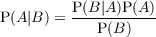 Laplace [1814] independently rediscovered Bayes’ theorem and published the work of
inductive reasoning by using probabilities. He presented “inverse probabilities”
(inferential statistics) allowing the study of causes by observing effects: the first use
of learning the probabilities of observations knowing states to then infer states having
only observations.
Laplace [1814] independently rediscovered Bayes’ theorem and published the work of
inductive reasoning by using probabilities. He presented “inverse probabilities”
(inferential statistics) allowing the study of causes by observing effects: the first use
of learning the probabilities of observations knowing states to then infer states having
only observations.
Later, by extending logic to plausible reasoning, Jaynes [2003] arrived at the same
properties than the theory of probability of Kolmogorov [1933]. Plausible reasoning
originates from logic, whose statements have degrees of plausibility represented by
real numbers. By turning rules of inferences into their probabilistic counterparts, the
links between logic and plausible reasoning are direct. With C = [A ⇒ B], we have:
- modus ponens, A entails B and A = true gives us B = false:
![[A-⇒-B-]∧-[A-=-true]
B = true](phdthesis19x.png) translates to
translates to
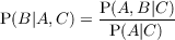 As P(A,B|C) = P(A|C) we have P(B|A,C) = 1
- modus tollens, A entails B and B = false gives us A = false (otherwise
B = true):
![[A ⇒-B]∧-[B-=-false]
A = false](phdthesis21x.png) translates to
translates to
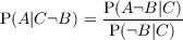 As P(A¬B|C) = 0 we have P(A|¬B,C) = 0, so P(¬A|¬B,C) = 1
Also, additionally to the two strong logic syllogisms above, plausible reasoning gets two
weak syllogisms, from:
-
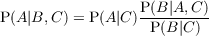 we get
![-[A-⇒-B-]∧-[B-=-true]--
A becomes more plausible](phdthesis24x.png) If A stands for “the enemy has done action a” and B for “the enemy is
doing action b”: “the enemy is doing b so it is more probable that she did
a beforehand (than if we knew nothing)”. Because there are only a (not
strict) subset of all the possible states (possibly all possible states) which
may lead in new states, when we are in these new states, the probability
of their origin states goes up.
If A stands for “the enemy has done action a” and B for “the enemy is
doing action b”: “the enemy is doing b so it is more probable that she did
a beforehand (than if we knew nothing)”. Because there are only a (not
strict) subset of all the possible states (possibly all possible states) which
may lead in new states, when we are in these new states, the probability
of their origin states goes up.
-
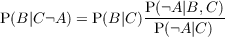 we get
![[A ⇒ B ]∧ [A = false]
B-becomes-less plausible](phdthesis26x.png) Using the same meanings for A and B as above: “the enemy has not
done a so it is less probable that she does b (than if we knew nothing)”.
Because there are only a (not strict) subset of all the possible states
(possibly all possible states) which may lead in new states, when we are
not in one of these origin states, there are less ways to go to new states.
Using the same meanings for A and B as above: “the enemy has not
done a so it is less probable that she does b (than if we knew nothing)”.
Because there are only a (not strict) subset of all the possible states
(possibly all possible states) which may lead in new states, when we are
not in one of these origin states, there are less ways to go to new states.
A reasoning mechanism needs to be consistent (one cannot prove A and ¬A at the
same time). For plausible reasoning, consistency means: a) all the possible ways to reach
a conclusion leads to the same result, b) information cannot be ignored, c) two equal
states of knowledge have the same plausibilities. Adding consistency to plausible
reasoning leads to Cox’s theorem [Cox, 1946], which derives the laws of probability:
the “product-rule” (P(A,B) = P(A ∩ B) = P(A|B)P(B)) and the “sum-rule”
(P(A + B) = P(A) + P(B) - P(A,B) or P(A ∪ B) = P(A) + P(B) - P(A ∩ B)) of
probabilities.
Indeed, this was proved by Cox [1946], producing Cox’s theorem (also named
Cox-Jayne’s theorem):
Theorem. A system for reasoning which satisfies:
- divisibility and comparability, the plausibility of a statement is a real
number,
- common sense, in presence of total information, reasoning is isomorphic
to Boolean logic,
- consistency, two identical mental states should have the same degrees of
plausibility,
is isomorphic to probability theory.
So, the degrees of belief, of any consistent induction mechanism, verify
Kolmogorov’s axioms. Finetti [1937] showed that if reasoning is made in a system
which is not isomorphic to probability theory, then it is always possible to find a
Dutch book (a set of bets which guarantees a profit regardless of the outcomes). In
our quest for a consistent reasoning mechanism which is able to deal with
(extensional and intentional) uncertainty, we are thus bound to
probability theory.
3.2.2 A formalism for Bayesian models
Inspired by plausible reasoning, we present Bayesian programming, a formalism that
can be used to describe entirely any kind of Bayesian model. It subsumes Bayesian
networks and Bayesian maps, as it is equivalent to probabilistic factor graphs Diard
et al. [2003]. There are mainly two parts in a Bayesian program (BP)*, the
description of how to compute the joint distribution, and the question(s) that it
will be asked.
The description consists in exhibiting the relevant variables {X1,…,Xn} and
explain their dependencies by decomposing the joint distribution P(X1…Xn|δ,π) with
existing preliminary (prior) knowledge π and data δ. The forms of each term of the
product specify how to compute their distributions: either parametric forms (laws or
probability tables, with free parameters that can be learned from data δ) or recursive
questions to other Bayesian programs.
Answering a question is computing the distribution P(Searched|Known), with
Searched and Known two disjoint subsets of the variables.
General Bayesian inference is practically intractable, but conditional
independence hypotheses and constraints (stated in the description) often
simplify the model. There are efficient ways to calculate the joint distribution
like message passing and junction tree algorithms [Pearl, 1988, Aji and
McEliece, 2000, Naïm et al., 2004, Mekhnacha et al., 2007, Koller and
Friedman, 2009]. Also, there are different well-known approximation techniques:
either by sampling with Monte-Carlo (and Monte-Carlo Markov Chains)
methods [MacKay, 2003, Andrieu et al., 2003], or by calculating on a simpler
(tractable) model which approximate the full joint as with variational Bayes
[Beal, 2003].
We sum-up the full model by what is called a Bayesian program, represented as:
For the use of Bayesian programming in sensory-motor systems, see [Bessière
et al., 2008]. For its use in cognitive modeling, see [Colas et al., 2010]. For its first
use in video game AI, applied to the first person shooter gameplay (Unreal
Tournament), see [Le Hy et al., 2004].
To sum-up, by using probabilities as an extension of propositional logic, the
method to build Bayesian models gets clearer: there is a strong parallel between
Bayesian programming and logic or declarative programming. In the same order as
the presentation of Bayesian programs, modeling consists in the following
steps:
-
1.
- Isolate the variables of the problem: it is the first prior that the
programmer puts into the system. The variables can be anything, from
existing input or output values of the problem to abstract/aggregative
values or parameters of the model. Discovering which variable to use for
a given problem is one of the most complicated form of machine learning.
-
2.
- Suppose and describe the influences and dependencies between these
variables. This is another prior that the programmer can have on the
problem, and learning the structure between these variables is the second
most complicated form of learning [François and Leray, 2004, Leray and
Francois, 2005].
-
3.
- Fill the priors and conditional probabilities parameters. The programmer
needs to be an expert of the problem to put relevant parameters, although
this is the easiest to learn from data once variables and structure are
specified. Learning the structure can be seen as learning the parameters
of a fully connected model and then removing dependencies where are the
less influent parameters.
In the following, we present how we applied this method to a simulated MMORPG*
fight situation as an example.
By following these steps, one may have to choose among several models. That is
not a problem as there are rational ground to make this choices, “all models are
wrong; some are useful” (George Box). Actually, the full question that we ask is
P(Searched|Known,π,δ), it depends on the modeling assumptions (π) as well as the
data (δ) that we used for training (if any). A simple way to view model
selection is to pick the model which makes the fewest assumptions (Occam’s
razor). In fact, Bayesian inference carries Occam’s razor with it: we shall ask
what is the plausibility of our model prior knowledge in the light of the data
P(π|δ).
Indeed, when evaluating two models π1 and π2, doing the ratio of evidences for
the two modeling assumption helps us choose:
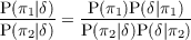 | (3.4) |
If our model is complicated, its expressiveness is higher, and so it can model more
complex causes of/explanations for the dataset. However, the probability mass will be
spread thiner on the space of possible datasets than for a simpler model. For
instance, in the task of regression, if π1 can only encode linear regression
(y = Ax + b) and π2 can also encore quadratic regression (y = Ax + Bx2 + c), all the
predictions for π1 are concentrated on linear (affine) functions, while for π2 the
probability mass of predictions is spread on more possible functions. If we only have
data δ of linear functions, the evidence for π1, P(π1|δ) will be higher. If δ
contains some quadratic functions, the evidence ratio will shift towards π2 as
the second model has better predictions: the shift to π2 happens when the
additional model complexity of π2 and the prediction errors of π1 balance each
other.
3.3 Modeling of a Bayesian MMORPG player
3.3.1 Task
We will now present a model of a MMORPG* player with the Bayesian programming
framework [Synnaeve and Bessière, 2010]. A role-playing game (RPG) consist
in the incarnation by the human player of an avatar with specific skills,
items, numbers of health points (HP) and stamina or mana (magic energy)
points (we already presented this gameplay in section 2.6). We want to
program a robotic player which we can substitute to a human player in a
battle scenario. More specifically here, we modeled the “druid” class, which is
complex because it can cast spells to deal damages or other negative effects as
well as to heal allies or enhance their capacities (“buff” them). The model
described here deals only with a sub-task of a global AI for autonomous
NPC.
The problem that we try to solve is: how do we choose which skill to use, and on
which target, in a PvE* battle? The possible targets are all our allies and foes. There
are also several skills that we can use. We will elaborate a model taking all our
perceptions into account and giving back a distribution over possible
target and skills. We can then pick the most probable combination that is yet
possible to achieve (enough energy/mana, no cooldown/reload time) or simply
sample in this distribution.
An example of a task that we have to solve is depicted in Figure 3.2, which shows
two different setups (states) of the same scenario: red characters are foes, green ones
are allies, we control the blue one. The “Lich” is inflicting damages to the “MT”
(main tank), the “Add” is hitting the “Tank”. In setup A, only the “Tank” is
near death, while in setup B both the “Tank” and the “Add” are almost
dead. A first approach to reason about these kind of situations would be
to use the combination of simple rules and try to give them some priority.
- if an ally has less than X (threshold) HP then use a “heal” on him.
- if the enemy receiving most damage has resistances (possibly in a list),
lower them if possible.
- if allies (possibly in a list) are not “buffed” (enhanced), buff them if
possible.
- default: shoot at the most targeted enemy.
- self-preservation, etc.
The problem with such an approach is that tuning or modifying it can quickly be
cumbersome: for a game with a large state space, robustness is hard to ensure. Also,
the behavior would seem pretty repetitive, and thus predictable.
3.3.2 Perceptions and actions
To solve this problem without having the downsides of this naive first approach, we
will use a Bayesian model. We now list some of the perceptions available to the player
(and thus the robot):
- the names and positions of all other players, this gives their distances,
which is useful to know which abilities can be used.
- hit points (also health points, noted HP) of all the players, when the HP
of a player fall to 0, her avatar dies. It cannot be resurrected, at least in
the situations that we consider (not for the fight).
- the natures of other players (ally or foe).
- the class of other players: some have a tanking role (take incoming damages
for the rest of the group), others are damage dealers (either by contact or
ranged attacks), the last category are healers, whose role is to maintain
everyone alive.
- an approximation of the resistance to certain types of attacks for every
player.
Actions available to the players are to move and to use their abilities:
- damage over time attacks (periodic repeated damage), or quick but low
damage attacks, and slow but high damage attacks
- energy/mana/stamina regenerators
- heal over time (periodic heal to selected allies), or quick but small heals,
and slow but big heals
- immobilizations, disabling effects (“stun”)
- enhancement of the selected allies HP/attack/speed... and crippling
attacks (enhancing future attacks), maledictions
- removing maledictions...
Here, we consider that the choice of a target and an ability to use on it strongly
condition the movements of the player, so we will not deal with moving the
character.
3.3.3 Bayesian model
We recall that write a Bayesian model by first describing the variables, their relations
(the decomposition of the join probability), and the forms of the distribution. Then
we explain how we identified the parameters and finally give the questions that will
be asked.
Variables
A simple set of variables is as follows:
- Target: Tt-1,t ∈ {t1…tn} at t and t - 1 (previous action). Tt is also
abusively noted T in the rest of the model. We have the n characters
as possible targets; each of them has their own properties variables (the
subscripting in the following variables).
- Hit Points: HPi∈⟦1…n⟧ ∈ [0…9] is the hit points value of the ith player.
Health/Hit points (HP) are discretized in 10 levels, from the lower to the
higher.
- Distance: Di∈⟦1…n⟧ ∈ {Contact,Close,Far,V eryFar} is the distance of
the ith player to our robotic character. Distance (D) is discretized in
4 zones around the robot character: contact where it can attack with a
contact weapon, close, far and (very far) to the further for which we have
to move even for shooting the longest distance weapon/spell.
- Ally: Ai∈⟦1…n⟧∈{true,false} is true is the ith player is an ally, and false
otherwise.
- Derivative Hit Points: ΔHPi∈⟦1…n⟧ ∈ {-,0,+} (decreasing, stable,
increasing) is the evolution of the hit points of the ith player. ΔHP is
a 3-valued interpolated value from the previous few seconds of fight that
informs about the ith character getting wounded or healed (or nothing).
- Imminent Death: IDi∈⟦1…n⟧ ∈ {true,false} tells if the ith player is in
danger of death. Imminent death (ID) is an interpolated value that
encodes HP, ΔHP and incoming attacks/attackers. This is a Boolean
variable saying if the ith character if going to die anytime soon. This is an
example of what we consider that an experienced human player will infer
automatically from the screen and notifications.
- Class: Ci∈⟦1…n ∈{Tank,Contact,Ranged,Healer} is the class of the ith
player. Class (C) is simplified over 4 values: a Tank can take a lot of
damages and taunt enemies, a Contact class which can deal huge amounts
of damage with contact weapons (rogue, barbarian...), Ranged stands for
the class that deals damages from far away (hunters, mages...) and Healers
are classes that can heal in considerable amounts.
- Resists:
Ri∈⟦1…n⟧ ∈ {Nothing,Fire,Ice,Nature,FireIce,IceNat,FireNat,All}
informs about the resistances of the ith player. The resist variable is the
combination of binary variables of resistance to certain types of (magical)
damages into one variable. With 3 possible resistances we get (23) 8
possible values. For instance “Ri = FireNat” means that the ith character
resists fire and nature-based damages. Armor (physical damages) could
have been included, and the variables could have been separated.
- Skill: S ∈{Skill1…Skillm}. The skill variable takes all the possible skills
for the given character, and not only the available ones to cast at the
moment to be able to have reusable probability tables (i.e. it is invariant
of the dynamics of the game).
Decomposition
The joint distribution of the model is:
We want to compute the probability distribution on the variable target (T) and skill
(S), so we have to consider the joint distribution with all variables on which target
(T) or skill (S) are conditionally dependent: the previous value of target (Tt-1), and
all the perceptions variables on each character.
- The probability of a given target depends on the previous one (it encodes
the previous decision and so all previous states).
- The health (or hit) points (HPi) depends on the facts that the ith
character is an ally (Ai), on his class (Ci), and if he is a target (T). Such a
conditional probability table should be learned, but we can already foresee
that a targeted ally with a tanking class (C = tank) would have a high
probability of having low hit points (HP) because taking it for target
means that we intend to heal him.
- The distance of the unit i (Di) is more probably far if unit i is an enemy
(Ai = false) and we target it (T = i) as our kind of druid attacks with
ranged spells and does not fare well in the middle of the battlefield.
- The probability of the ith character being an ally depends on if we target
allies of foes more often: that is P(Ai|S,T) encodes our propensity to
target allies (with heals and enhancements) or foes (with damaging or
crippling abilities).
- The probability that the ith units is losing hit points (ΔHPi = minus)
is higher for foes (Ai = false) with vulnerable classes (Ci = healer) that
are more susceptible to be targeted (T = i), and also for allies (Ai = true)
whose role is to take most of the damages (Ci = tank). As for Ai, the
probability of IDi is driven by our
- Obviously, the usage of skills depends on their efficiency on the target
(R, resistances), and on their class. As a result, we have P(Ri|Ci,S,T) as
the conditional distribution on “resists”. The probability of the resist to
“nature based effects” (Ri = nature) for skills involving “nature” damage
(s ∈{nature_damage}) will be very low as it will be useless to use spells
that the receiver is protected against.
- The probability that the ith character will die soon (IDi) will be high if
i is targeted (T = i) with a big heal or big instant damage (S = big_heal
or S = big_damage, depending on whether i is an ally or not).
Parameters
- P(Tt-1) is unknown and unspecified (uniform). In the question, we always
know what was the previous target, except when there was not one (at
the beginning).
- P(T|Tt-1) is a probability corresponding to the propensity to switch
targets. It can be learned, or uniform if there is no previous target (it the
prior on the targets then).
- P(S) is unknown and so unspecified, it could be a prior on the preferred
skills (for style of for efficiency).
- P(HPi|Ai,Ci,S,T) is a 2 × 4 ×m× 2 probability table, indexed on if the
ith character is an ally or not, on its class, on the skills (#S = m) and on
where it is the target or not. It can be learned (and/or parametrized), for
instance P(HPi = x|ai,ci,s,t) =
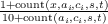 .
.
- P(Di|Ai,S,T) is a 4 × 2 × m × 2 (possibly learned) probability table.
- P(Ai|S,T) is a 2 × m × 2 (possibly learned) probability table.
- P(ΔHPi|Ai,S,T) is a 3 × 2 × m × 2 (possibly learned) probability table.
- P(Ri|Ci,S,T) is a 8 × 4 × m × 2 (possibly learned) probability table.
- P(Ci|Ai,S,T) is a 4 × 2 × m × 2 (possibly learned) probability table.
Identification
In the following Results part however, we did not apply learning but instead
manually specified the probability tables to show the effects of gamers’ common sense
rules and how it/they can be correctly encoded in this model.
About learning: if there were only perceived variables, learning the right
conditional probability tables would just be counting and averaging. However, some
variables encode combinations of perceptions and passed states. We could learn such
parameters through the EM algorithm but we propose something simpler for the
moment as our “not directly observed variables” are not complex to compute, we
compute them from perceptions as the same time as we learn. For instance we map
in-game values to their discrete values for each variables online and only store the
resulting state “compression”.
Questions
In any case, we ask our (updated) model the distribution on S and T knowing all the
state variables:
 | (3.8) |
We then proceed to choose to do the highest scoring combination of S ∧T that is
available (skills may have cooldowns or cost more mana/energy that we have
available).
As (Bayes rule) P(S,T) = P(S|T).P(T), if we want to decompose this question,
we can ask:
 Which means that we want to know the distribution on T knowing all the
relevant state variables, followed by (with the newly computed distribution on
T):
Which means that we want to know the distribution on T knowing all the
relevant state variables, followed by (with the newly computed distribution on
T):
 in which we use this distribution on T to compute the distribution on S
with:
in which we use this distribution on T to compute the distribution on S
with:
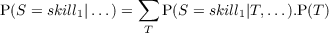 We here choose to sum over all possible values of T. Note that we did not
ask:
We here choose to sum over all possible values of T. Note that we did not
ask:
P(S|T = most_probable,…) but computed instead

Bayesian program
Here is the full Bayesian program corresponding to this model:
3.3.4 Example
This model has been applied to a simulated situation with 2 foes and 4 allies while
our robot took the part of a druid. We display a schema of this situation in
Figure 3.2. The arrows indicate foes attacks on allies. HOT stands for heal over time,
DOT for damage over time, “abol” for abolition and “regen” for regeneration, a “buff”
is an enhancement and a “dd” is a direct damage. “Root” is a spell which prevents the
target from moving for a short period of time, useful to flee or to put some distance
between the enemy and the druid to cast attack spells. “Small” spells are usually
faster to cast than “big” spells. The difference between setup A and setup
B is simply to test the concurrency between healing and dealing damage
and the changes in behavior if the player can lower the menace (damage
dealer).

To keep things simple and because we wanted to analyze the answers of the
model, we worked with manually defined probability tables.In the experiments, we
will try different values P(IDi|T = i), and see how the behavior of the agent
changes.
We set the probability to target the same target as before (P(Tt = i|Tt-1 = i)) to
0.4 and the previous target to “Lich” so that the prior probability for all other
6 targets is 0.1 (4 times more chances to target the Lich than any other
character).
We set the probability to target an enemy (instead of an ally) P(Ai = false|T = i) to
0.6. This means that our Druid is mainly a damage dealer and just a backup
healer.
When we only ask what the target should be:
 We
can see on Figure 3.3 (left) that the evolution from selecting the main foe “Lich” to
selecting the ally “Tank” is driven by the increase of the probability that the selected
target is near death, and our robot eventually moves on targeting their “Tank” ally
(to heal them). We can see on Figure 3.3 (right) that, at some point, our robot
prefers to kill the dying “add” (additional foe) to save their ally Tank instead of
healing them. Note that there is no variable showing the relation between
“Add” and “Tank” (the first is attacking the second, who is taking damages
from the first), but this could be taken into account in a more complete
model.
We
can see on Figure 3.3 (left) that the evolution from selecting the main foe “Lich” to
selecting the ally “Tank” is driven by the increase of the probability that the selected
target is near death, and our robot eventually moves on targeting their “Tank” ally
(to heal them). We can see on Figure 3.3 (right) that, at some point, our robot
prefers to kill the dying “add” (additional foe) to save their ally Tank instead of
healing them. Note that there is no variable showing the relation between
“Add” and “Tank” (the first is attacking the second, who is taking damages
from the first), but this could be taken into account in a more complete
model.
When we ask what skill we should use:
 We
can see on Figure 3.4 the influence of imminent death (IDi) on skill (S) which is
coherent with the target distribution:
We
can see on Figure 3.4 the influence of imminent death (IDi) on skill (S) which is
coherent with the target distribution:
- in setup A (left), we evolve with the increase of P(IDi = true|T = i) to
choose to heal (our ally),
- in setup B (right), to deal direct damage (and hopefully, kill) the foe
attacking our ally.
As you can see here, when we have the highest probability to attack the main enemy
(“Lich”, when P(IDi = true|T = i) is low), who is a C = tank, we get a
high probability for the skill debuff_armor. We need only cast this skill if
the debuff is not already present, so perhaps that we will cast small_dd
instead.
To conclude this example, we ask the full question, what is the distribution on
skill and target:
 Figure 3.5 shows this distribution with setup A and the probability to target the
previous target (set to “Lich” here) only ≈ 2 times greater than any other character,
P(IDi = true|T = i) = 0.9 and P(Ai = false|T = i) = 0.6. To make decisions about
our actions, a simple approach would be a greedy one: if the first couple (T,S) is
already done or not available, we perform the second, and so on. Another approach
would be to sample in this distribution.
Figure 3.5 shows this distribution with setup A and the probability to target the
previous target (set to “Lich” here) only ≈ 2 times greater than any other character,
P(IDi = true|T = i) = 0.9 and P(Ai = false|T = i) = 0.6. To make decisions about
our actions, a simple approach would be a greedy one: if the first couple (T,S) is
already done or not available, we perform the second, and so on. Another approach
would be to sample in this distribution.
3.3.5 Discussion
This limited model served the purpose of presenting Bayesian programming in
practice. While it was used in a simulation, it showcases the approach one can take to
break down the problem of autonomous control of NPC*. The choice of the skill or
ability to use and the target on which to use it puts hard constraints on every others
decisions the autonomous agent has to take to perform its ability action. Thus, such
a model shows that:
- cooperative behavior is not too hard to incorporate in a decision (instead
of being hard-coded),
- it can be learned, either from observations of a human player or by
reinforcement (exploration),
- it is computationally tractable (for use in all games).
Moreover, using this model on another agent than the one controlled by the AI can give
a prediction on what it will do, resulting in human-like, adaptive, playing
style.
We did not kept at the research track of Bayesian modeling MMORPG games due
to the difficulty to work on these types of games: the studios have too much to lose to
“farmer” bots to accept any automated access to the game. Also, there are no sharing
format of data (like replays) and the invariants of the game situations are fewer
than in RTS games. Finally, RTS games have international AI competitions
which were a good motivation to compare our approach with other game AI
researchers.
Chapter 4
RTS AI: StarCraft: Broodwar
We think of life as a journey with a destination (success, heaven). But
we missed the point. It was a musical thing, we were supposed to sing and
dance while music was being played.
|
THIS chapter explains the basics of RTS gameplay*, particularly of StarCraft.
We then list the (computational) challenges brought by RTS gameplay. We
present a transversal decomposition of the RTS AI domain in levels of abstractions
(strategy, tactics, micro-management*), which we will use for the rest of the
dissertation.
4.1 How does the game work
4.1.1 RTS gameplay
We first introduce the basic components of a real-time strategy (RTS) game. The
player is usually referred as the “commander” and perceives the world in an
allocentric “God’s view”, performing mouse and keyboard actions to give orders to
units (or squads of units) within a circumvented area (the “map”). In a RTS, players
need to gather resources to build military units and defeat their opponents. To that
end, they often have worker units (or extraction structures) that can gather
resources needed to build workers, buildings, military units and research
upgrades. Workers are often also builders (as in StarCraft) and are weak in
fights compared to military units. Resources may have different uses, for
instance in StarCraft: minerals* are used for everything, whereas gas* is only
required for advanced buildings or military units, and technology upgrades.
Buildings and research upgrades define technology trees (directed acyclic graphs)
and each state of a tech tree* (or build tree*) allow for different unit type
production abilities and unit spells/abilities. The military units can be of
different types, any combinations of ranged, casters, contact attack, zone
attacks, big, small, slow, fast, invisible, flying... In the end, a central part of
the gameplay is that units can have attacks and defenses that counter each
others as in a soft rock-paper-scissors. Also, from a player point of view,
most RTS games are only partially observable due to the fog of war* which
hides units and new buildings which are not in sight range of the player’s
units.
In chronological order, RTS include (but are not limited to): Ancient Art of War,
Herzog Zwei, Dune II, Warcraft, Command & Conquer, Warcraft II, C&C: Red
Alert, Total Annihilation, Age of Empires, StarCraft, Age of Empires II, Tzar,
Cossacks, Homeworld, Battle Realms, Ground Control, Spring Engine games,
Warcraft III, Total War, Warhammer 40k, Sins of a Solar Empire, Supreme
Commander, StarCraft II. The differences in gameplay are in the order of number,
nature and gathering methods of resources; along with construction, research
and production mechanics. The duration of games vary from 15 minutes for
the fastest to (1-3) hours for the ones with the biggest maps and longest
gameplays. We will now focus on StarCraft, on which our robotic player is
implemented.
4.1.2 A StarCraft game
StarCraft is a science-fiction RTS game released by Blizzard EntertainmentTM in
March 1998. It was quickly expanded into StarCraft: Brood War (SC: BW) in
November 1998. In the following, when referring to StarCraft, we mean StarCraft
with the Brood War expansion. StarCraft is a canonical RTS game in the sense that
it helped define the genre and most gameplay* mechanics seen in other RTS games
are present in StarCraft. It is as much based on strategy than tactics, by
opposition to the Age of Empires and Total Annihilation series in which
strategy is prevalent. In the following of the thesis, we will focus on duel
mode, also known as 1 vs. 1 (1v1). Team-play (2v2 and higher) and “free
for all” are very interesting but were not studied in the framework of this
research. These game modes particularly add a layer of coordination and bluff
respectively.
A competitive game
StarCraft sold 9.5 millions licenses worldwide, 4.5 millions in South Korea alone
[Olsen, 2007], and reigned on competitive RTS tournaments for more than a decade.
Numerous international competitions (World Cyber Games, Electronic Sports
World Cup, BlizzCon, OnGameNet StarLeague, MBCGame StarLeague)
and professional gaming (mainly in South Korea [Chee, 2005]) produced a
massive amount of data of highly skilled human players. In South Korea,
there are two TV channels dedicated to broadcasting competitive video
games, particularly StarCraft. The average salary of a pro-gamer* there
was up to 4 times the average South Korean salary [MYM, 2007] (up to
$200,000/year on contract for NaDa). Professional gamers perform about
300 actions (mouse and keyboard clicks) per minute while following and
adapting their strategies, while their hearts reach 160 beats per minute (BPM
are displayed live in some tournaments). StarCraft II is currently (2012)
taking over StarCraft in competitive gaming but a) there is still a strong pool
of highly skilled StarCraft players and b) StarCraft II has a really similar
gameplay.
Replays
StarCraft (like most RTS) has a replay* mechanism, which enables to record every
player’s actions such that the state of the game can be deterministically re-simulated.
An extract of a replay is shown in appendix in Table B.1. The only piece of
stochasticity comes from “attack miss rates” (≈ 47%) when a unit is on a lower
ground than its target. These randomness generator seed is saved along with the
actions in the replay. All high level players use this feature heavily either to improve
their play or study opponents’ styles. Observing replays allows player to see what
happened under the fog of war*, so that they can understand timing of technologies
and attacks, and find clues/evidences leading to infer the strategy as well as weak
points.
Factions
In StarCraft, there are three factions with very different units and technology trees:
- Terran: humans with strong defensive capabilities and balanced, averagely
priced biological and mechanical units.
- Protoss: advanced psionic aliens with expensive, slow to produce and
resistant units.
- Zerg: insectoid alien race with cheap, quick to produce and weak units.
The races are so different that learning to play a new race competitively is almost like
learning to play with new rules.
Economy
All factions use workers to gather resources, and all other characteristics are different:
from military units to “tech trees*”, gameplay styles. Races are so different that
highly skilled players focus on playing with a single race (but against all
three others). There are two types of resources, often located close together,
minerals* and gas*. From minerals, one can build basic buildings and units,
which opens the path to more advanced buildings, technologies and units,
which will in turn all require gas to be produced. While minerals can be
gathered at an increasing rate the more workers are put at work (asymptotically
bounded) , the gas gathering rate is quickly limited to 3 workers per gas
geyser (i.e. per base). There is another third type of “special” resource, called
supply*, which is the current population of a given player (or the cost in
population of a given unit), and max supply*, which is the current limit of
population a player can control. Max supply* can be upgraded by building special
buildings (Protoss Pylon, Terran Supply Depot) or units (Zerg Overlord),
giving 9 to 10 additional max supply*, up to a hard limit of 200. Some units
cost more supply than others (from 0.5 for a Zergling to 8 for a Protoss
Carrier or Terran Battlecruiser). In Figure 4.1, we show the very basics of
Protoss economy and buildings. Supply will sometimes be written supply/max
supply (supply on max supply). For instance 4/9 is that we currently have a
population of 4 (either 4 units of 1, or 2 of 2 or ...) on a current maximum of
9.
Openings and strategy
To reach a competitive amateur level, players have to study openings* and hone their
build orders*. An opening corresponds to the first strategic moves of a game, as in
other abstract strategy games (Chess, Go). They are classified/labeled with names
from high level players. A build-order is a formally described and accurately
timed sequence of buildings to construct in the beginning. As there is a
bijection between optimal population and time (in the beginning, before any
fight), build orders are indexed on the total population of the player as in the
example for Protoss in table 4.1. At the highest levels of play, StarCraft games
usually last between 6 (shortest games, with a successful rush from one of the
player) to 30 minutes (long economically and technologically developed game).
|
|
|
| Supply/Max supply | Build | Note |
| (population/max) | or Product | |
|
|
|
| 8/9 | Pylon | “supply/psi/control/population” building |
| 10/17 | Gateway | units producing structure |
| 12/17 | Assimilator | constructed on a gas geyser, to gather gas |
| 14/17 | Cybernetics Core | technological building |
| 16/17 | Pylon | “supply/psi/control/population” building |
| 16/17 | Range | it is a research/tech |
| 17/25 | Dragoon | first military unit |
|
|
|
| |
Table 4.1: An example of the beginning of a “2 Gates Goon Range” Protoss
build order which focus on building dragoons and their attack range upgrade
quickly.
A commented game
We now present the evolution of a game (Figures 4.2 and 4.3) during which
we tried to follow the build order presented in table 4.1 (“2 Gates Goon
Range” )
but we had to adapt to the fact that the opponent was Zerg (possibility for a faster
rush) by building a Gateway at 9 supply and building a Zealot (ground contact unit)
before the first Dragoon. The first screenshot (image 1 in Figure 4.2) is at the very
start of the game: 4 Probes (Protoss workers), and one Nexus (Protoss main building,
producing workers and depot point for resources). At this point players have to
think about what openings* they will use. Should we be aggressive early
on or opt for a more defensive opening? Should we specialize our army for
focused tactics, to the detriment of being able to handle situations (tactics and
armies compositions) from the opponent that we did not foresee? In picture
2 in the same Figure (4.2), the first gate is being built. At this moment,
players often send a worker to “scout” the enemy’s base, as they cannot have
military units yet, it is a safe way to discover where they are and inquiry about
what they are doing. In picture 3, the player scouts their opponent, thus
gathering the first bits of information about their early tech tree. Thus,
knowing to be safe from an early attack (“rush”), the player decides to go for
a defensive and economical strategy for now. Picture 4 shows the player
“expanding”, which is the act of making another base at a new resource
location, for economical purposes. In picture 5, we can see the upgrading of the
ground weapons along with 4 ranged military units, staying in defense at the
expansion. This is a technological decision of losing a little of potential “quick
military power” (from military units which could have been produced for this
minerals and gas) in exchange of global upgrade for all units (alive and to be
produced), for the whole game. This is an investment in both resources
and time. Picture 6 showcases the production queue of a Gateway as well
as workers transferring to a second expansion (third base). Being safe and
having expanded his tech tree* to a point where the army composition is
well-rounded, the player opted for a strategy to win by profiting from an
economical lead. Figure 4.3 shows the aggressive moves of the same player:
in picture 7, we can see a flying transport with artillery and area of effect
“casters” in it. The goal of such an attack is not to win the game right away
but to weaken the enemy’s economy: each lost worker has to be produced,
and, mainly, the missing gathering time adds up quite quickly. In picture 8,
the transport in unloaded directly inside the enemy’s base, causing huge
damages to their economy (killing workers, Zerg Drones). This is the use of a
specialized tactics, which can change the course of a game. At the same time, it
involves only few units (a flying transport and its cargo), allowing for the
main army to stay in defense at base. It capitalizes on the manoeuverability
of the flying Protoss Shuttle, on the technological advancements allowing
area of effects attacks and the large zone that the opponent has to cover to
defend against it. In picture 9, an invisible attacking unit (circled in white) is
harassing the oblivious enemy’s army. This is an example of how technology
advance on the opponent can be game changing (the opponent does not have
detection in range, thus is vulnerable to cloaked units). Finally, picture 10
shows the final attack, with a full ground army marching on the enemy’s
base.
4.2 RTS AI challenges
In combinatorial game theory terms, competitive StarCraft (1 versus 1) is a zero sum, partial-information,
deterministic
strategy game. StarCraft subsumes Wargus (Warcraft II open source clone), which
has an estimated mean branching factor 1.5.103 [Aha et al., 2005] (Chess: ≈ 35, Go:
< 360): Weber [2012] finds a branching factor greater than 1.106 for StarCraft. In a
given game (with maximum map size) the number of possible positions is roughly of
1011500, versus the Shannon number for Chess (1043) [Shannon, 1950]. Also, we
believe strategies are much more balanced in StarCraft than in most other
games. Otherwise, how could it be that more than a decade of professional
gaming on StarCraft did not converge to a finite set of fixed (imbalanced)
strategies?
Humans deal with this complexity by abstracting away strategy from low
level actions: there are some highly restrictive constraints on where it is
efficient (“optimal”) to place economical main buildings (Protoss Nexus, Terran
Command Center, Zerg Hatchery/Lair/Hive) close to minerals spots and
gas geysers. Low-level micro-management* decisions have high horizontal
continuity and humans see these tasks more like playing a musical instrument
skillfully. Finally, the continuum of strategies is analyzed by players and
some distinct strategies are identified as some kinds of “invariants”, or “entry
points” or “principal components”. From there, strategic decisions impose some
(sometimes hard) constraints on the possible tactics, and the complexity is
broken by considering only the interesting state space due to this high vertical
continuity.
Most challenges of RTS games have been identified by [Buro, 2003, 2004]. We
will try to anchor them in the human reasoning that goes on while playing a
StarCraft game.
- Adversarial planning under uncertainty
(along with resource management): it diverges from traditional planning
under uncertainty in the fact that the player also has to plan against the
opponent’s strategy, tactics, and actions. From the human point of view,
he has to plan for which buildings to build to follow a chosen opening*
and subsequent strategies, under a restricted resources (and time) budget.
At a lower level, and less obvious for humans, are the plans they make to
coordinate units movements.
- Learning and opponent modeling, Buro accurately points out that human
players need very few (“a couple of”) games to spot their opponents’
weaknesses. Somehow, human opponent modeling is related to the
“induction scandal”, as Russell called it: how do humans learn so much
so fast? We learn from our mistakes, we learn the “play style” of our
opponent’s, we are quickly able to ask ourselves: “what should I do now
given what I have seen and the fact that I am playing against player
XYZ?”. “Could they make the same attack as last time?”. To this end, we
use high level representations of the states and the actions with compressed
invariants, causes and effects.
- Spatial and temporal reasoning (along with decision making under
uncertainty), this is related to planning under uncertainty but focuses on
the special relations between what can and what cannot be done in a given
time. Sadly, it was true in 2004 but is still true today: “RTS game AI [...]
falls victim to simple common-sense reasoning”. Humans learn sequences
of actions, and reason only about actions coherent with common sense.
For AI of complex systems, this common-sense is hard to encode and to
use.
- Collaboration (teamplay), which we will not deal with here: a lot has to
do with efficient communication and “teammate modeling”.
As we have seen previously more generally for multi-player video games, all these
challenges can be handled by Bayesian modeling. While acknowledging these
challenges for RTS AI, we now propose a different task decomposition, in which
different tasks will solve some parts of these problems at their respective
levels.
4.3 Tasks decomposition and linking
We decided to decompose RTS AI in the three levels which are used by the
gamers to describe the games: strategy, tactics, micro-management. We remind the
reader that parts of the map not in the sight range of the player’s units
are under fog of war*, so the player has only partial information about the
enemy buildings and army. The way by which we expand the tech tree, the
specific units composing the army, and the general stance (aggressive or
defensive) constitute what we call strategy. At the lower level, the actions
performed by the player (human or not) to optimize the effectiveness of
its units is called micro-management*. In between lies tactics: where to
attack, and how. A good human player takes much data in consideration
when choosing: are there flaws in the defense? Which spot is more worthy to
attack? How much am I vulnerable for attacking here? Is the terrain (height,
chokes) to my advantage? The concept of strategy is a little more abstract:
at the beginning of the game, it is closely tied to the build order and the
intention of the first few moves and is called the opening, as in Chess. Then, the
long term strategy can be partially summed up by three signals/indicators:
- aggression: how much is the player aggressive or defensive?
- initiative: how much is the player adapting to the opponent’s strategy vs.
how much is the player being original?
- technology/production/economy (tech/army/eco)
distribution of resources: how much is the player spending (relatively) in
these three domains?
At high levels of play, the tech/army/eco balance is putting a hard constraint on the
aggression and initiative directions: if a player invested heavily in their army
production, they should attack soon to leverage this investment. To the contrary, all
other things being equal, when a player expands*, they are being weak until the
expansion repaid itself, so they should play defensively. Finally, there are some
technologies (researches or upgrades) which unlocks an “attack timing” or “attack
window”, for instance when a player unlocks an invisible technology (or unit)
before that the opponent has detection technology (detectors). On the other
hand, while “teching” (researching technologies or expanding the tech tree*),
particularly when there are many intermediate technological steps, the player is
vulnerable because of the immediate investment they made, which did not pay off
yet.
From this RTS domain tasks decomposition, we can draw the mind map
given in Figure 4.4. We also characterized these levels of abstractions by:
- the conditioning that the decisions on one abstraction level have on the
other, as discussed above: strategy conditions tactics which conditions
low-level actions (that does not mean than there cannot be some feedback
going up the hierarchy).
- the quantity of direct information that a player can hope to get on
the choices of their opponent. While a player can see directly the
micro-management of their enemy (movements of units on the battlefront),
they cannot observe all the tactics, and a big part of tactics gameplay
is to hide or fake them well. Moreover, key technological buildings are
sometimes hidden, and the player has to form beliefs about the long term
strategy of the opponent (without being in their head).
- the time which is required to switch behaviors of a given level. For instance
a change of strategy will require to either a) (technology) build at least
two buildings or a building and a research/upgrade, b) (army) build
a few units, c) take a new expansion (new base). A change of tactics
corresponds to a large repositioning of the army(ies), while a change in
micro-management is very quick (like moving units out of an area-of-effect
damage zone).
This is shown in Figure 4.5. We will discuss the state of the art for the each
of these subproblems (and the challenges listed above) in their respective
parts.
To conclude, we will now present our works on these domains in separate
chapters:
- Micro-management: chapter 5,
- Tactics: chapter 6,
- Strategy: chapter 7,
- Robotic player (bot): chapter 8.
In Figure 4.6, we present the flow of informations between the different inference and
decision-making parts of the bot architecture. One can also view this problem as
having a good model of one’s strategy, one’s opponent strategy, and taking decisions.
The software architecture that we propose is to have services building and
maintaining the model of the enemy as well as our state, and decision-making
modules using all this information to give orders to actuators (filled in gray in
Fig. 4.6).
Chapter 5
Micro-management
La vie est la somme de tous vos choix.
Life is the sum of all your choices.
|
WE present a Bayesian sensory-motor model for multi-agent (decentralized)
units control in an adversarial setting. Orders, coming from higher up in the
decision hierarchy, are integrated as another sensory input. We first present the task
of units control, its challenges and previous works on the problem. We then introduce
all the perceptions and actions used before laying out our Bayesian model.
Finally, we evaluated our model on classic StarCraft micro-management*
tasks.
This work was published at Computational Intelligence in Games (IEEE CIG)
2011 in Seoul [Synnaeve and Bessière, 2011a].
- Problem: optimal control of units in a (real-time) huge adversarial actions
space (collisions, accelerations, terrain, damages, areas of effects, foes,
goals...).
- Problem that we solve: efficient coordinated control of units incorporating
all low level actions and inputs, plus higher level orders and
representations.
- Type: it is a problem of multi-agent control in an adversarial
environment .
- Complexity: PSPACE-complete [Papadimitriou and
Tsitsiklis, 1987, Viglietta, 2012]. Our solutions are real-time on a laptop.
5.1 Units management
5.1.1 Micro-management complexity
In this part, we focus on micro-management*, which is the lower-level in our
hierarchy of decision-making levels (see Fig. 4.5) and directly affect units
control/inputs. Micro-management consists in maximizing the effectiveness of the
units i.e. the damages given/damages received ratio. These has to be performed
simultaneously for units of different types, in complex battles, and possibly on
heterogeneous terrain. For instance: retreat and save a wounded unit so that the
enemy units would have to chase it either boosts your firepower (if you save the unit)
or weakens the opponent’s (if they chase).
StarCraft micro-management involves ground, flying, ranged, contact, static,
moving (at different speeds), small and big units (see Figure 5.2). Units may also
have splash damage, spells, and different types of damages whose amount will depend
on the target size. It yields a rich states space and needs control to be very fast:
human progamers can perform up to 400 “actions per minute” in intense fights.
The problem for them is to know which actions are effective and the most
rewarding to spend their actions efficiently. A robot does not have such physical
limitations, but yet, badly chosen actions have negative influence on the issue of
fights.
Let U be the set of the m units to control, A = {∪i  }∪S be the set of possible
actions (all n possible
}∪S be the set of possible
actions (all n possible  directions, standing ground included, and Skills, firing
included), and E the set of enemies. As |U| = m, we have |A|m possible
combinations each turn, and the enemy has |A||E|. The dimension of the set of
possible actions each micro-turn (for instance: 1/24th of a second in StarCraft)
constrains reasoning about the state of the game to be hierarchical, with
different levels of granularity. In most RTS games, a unit can go (at least) in
its 24 surrounding tiles (see Figure 5.2, each arrow correspond to a
directions, standing ground included, and Skills, firing
included), and E the set of enemies. As |U| = m, we have |A|m possible
combinations each turn, and the enemy has |A||E|. The dimension of the set of
possible actions each micro-turn (for instance: 1/24th of a second in StarCraft)
constrains reasoning about the state of the game to be hierarchical, with
different levels of granularity. In most RTS games, a unit can go (at least) in
its 24 surrounding tiles (see Figure 5.2, each arrow correspond to a  ) )
stay where it is, attack, and sometimes cast different spells: which yields
more than 26 possible actions each turn. Even if we consider only 8 possible
directions, stay, and attack, with N units, there are 10N possible combinations
each turn (all units make a move each turn). As large battles in StarCraft
account for at least 20 units on each side, optimal units control hides in too
big a search space to be fully explored in real-time (sub-second reaction at
least) on normal hardware, even if we take only one decision per unit per
second.
) )
stay where it is, attack, and sometimes cast different spells: which yields
more than 26 possible actions each turn. Even if we consider only 8 possible
directions, stay, and attack, with N units, there are 10N possible combinations
each turn (all units make a move each turn). As large battles in StarCraft
account for at least 20 units on each side, optimal units control hides in too
big a search space to be fully explored in real-time (sub-second reaction at
least) on normal hardware, even if we take only one decision per unit per
second.
5.1.2 Our approach
Our full robot has separate agents types for separate tasks (strategy, tactics,
economy, army, as well as enemy estimations and predictions): the part that
interests us here, the unit control, is managed by Bayesian units directly. Their
objectives are set by military goal-wise atomic units group, themselves spawned
to achieve tactical goals (see Fig. 5.1). Units groups tune their Bayesian
units modes (scout, fight, move) and give them objectives as sensory inputs.
The Bayesian unit is the smallest entity and controls individual units as
sensory-motor robots according to the model described above. The only inter
Bayesian units communication about attacking targets is handled by a structure
shared at the units group level. This distributed sensory-motor model for
micro-management* is able to handle both the complexity of unit control and the
need of hierarchy (see Figure 5.1). We treat the units independently, thus
reducing the complexity (no communication between our “Bayesian units”), and
allowing to take higher-level orders into account along with local situation
handling. For instance: the tactical planner may decide to retreat, or go
through a choke under enemy fire, each Bayesian unit will have the higher-level
order as a sensory input, along with topography, foes and allies positions.
From its perception, our Bayesian robot [Lebeltel et al., 2004] can compute
the distribution over its motor control. The performances of our models
are evaluated against the original StarCraft AI and a reference AI (based
on our targeting heuristic): they have proved excellent in this benchmark
setup.
5.2 Related work
Technical solutions include finite states machines (FSM) [Rabin, 2002], genetic
algorithms (GA) [Ponsen and Spronck, 2004, Bakkes et al., 2004, Preuss
et al., 2010], reinforcement learning (RL) [Marthi et al., 2005, Madeira
et al., 2006], case-based reasoning (CBR) [Aha et al., 2005, Sharma et al., 2007],
continuous action models [Molineaux et al., 2008], reactive planning [Weber
et al., 2010b], upper confidence bounds tree (UCT) [Balla and Fern, 2009], potential
fields [Hagelbäck and Johansson, 2009], influence maps[Preuss et al., 2010], and
cognitive human-inspired models [Wintermute et al., 2007].
FSM are well-known and widely used for control tasks due to their efficiency and
implementation simplicity. However, they don’t allow for state sharing, which
increases the number of transitions to manage, and state storing, which
makes collaborative behavior hard to code [Cutumisu and Szafron, 2009].
Hierarchical FSM (HFSM) solve some of this problems (state sharing) and
evolved into behavior trees (BT, hybrids HFSM) [Isla, 2005] and behavior
multi-queues (resumable, better for animation) [Cutumisu and Szafron, 2009] that
conserved high performances. However, adaptability of behavior by parameters
learning is not the main focus of these models, and unit control is a task
that would require a huge amount of hand tuning of the behaviors to be
really efficient. Also, these architectures does not allow reasoning under
uncertainty, which helps dealing with local enemy and even allied units. Our agents
see local enemy (and allied) units but do not know what action they are
going to do. They could have perfect information about the allied units
intentions, but this would need extensive communication between all the
units.
Some interesting uses of reinforcement learning (RL)* [Sutton and Barto, 1998]
to RTS research are concurrent hierarchical (units Q-functions are combined higher
up) RL* [Marthi et al., 2005] to efficiently control units in a multi-effector system
fashion. Madeira et al. [2006] advocate the use of prior domain knowledge to allow
faster RL* learning and applied their work on a large scale (while being not as large
as StarCraft) turn-based strategy game. In real game setups, RL* models have to
deal with the fact that the state spaces to explore is enormous, so learning will be
slow or shallow. It also requires the structure of the game to be described in a partial
program (or often a partial Markov decision process) and a shape function [Marthi
et al., 2005]. RL can be seen as a transversal technique to learn parameters of an
underlying model, and this underlying behavioral model matters. Ponsen and
Spronck [2004] used evolutionary learning techniques, but face the same problem of
dimensionality.
Case-based reasoning (CBR) allows for learning against dynamic opponents [Aha
et al., 2005] and has been applied successfully to strategic and tactical planning
down to execution through behavior reasoning rules [Ontañón et al., 2007a]. CBR
limitations (as well as RL) include the necessary approximation of the world and the
difficulty to work with multi-scale goals and plans. These problems led respectively to
continuous action models [Molineaux et al., 2008]and reactive planning [Weber
et al., 2010b]. Continuous action models combine RL and CBR. Reactive planning
use a decomposition similar to hierarchical task networks [Hoang et al., 2005] in that
sub-plans can be changed at different granularity levels. Reactive planning
allows for multi-scale (hierarchical) goals/actions integration and has been
reported working on StarCraft, the main drawback is that it does not address
uncertainty and so can not simply deal with hidden information (both extensional
and intentional). Fully integrated FSM, BT, RL and CBR models all need
vertical integration of goals, which is not very flexible (except in reactive
planning).
Monte-Carlo planning [Chung et al., 2005] and upper Upper confidence bounds
tree (UCT) planning (coming from Go AI) [Balla and Fern, 2009] samples
through the (rigorously intractable) plans space by incrementally building
the actions tree through Monte-Carlo sampling. UCT for tactical assault
planning [Balla and Fern, 2009] in RTS does not require to encode human
knowledge (by opposition to Monte-Carlo planning) but it is too costly,
both in learning and running time, to go down to units control on RTS
problems. Our model subsumes potential fields [Hagelbäck and Johansson, 2009],
which are powerful and used in new generation RTS AI to handle threat, as
some of our Bayesian unit sensory inputs are based on potential damages
and tactical goodness (height for the moment) of positions. Hagelbäck and
Johansson [2008] presented a multi-agent potential fields based bot able to
deal with fog of war in the Tankbattle game. Avery et al. [2009] and Smith
et al. [2010] co-evolved influence map trees for spatial reasoning in RTS
games. Danielsiek et al. [2008] used influence maps to achieve intelligent
squad movement to flank the opponent in a RTS game. A drawback for
potential field-based techniques is the large number of parameters that has
to be tuned in order to achieve the desired behavior. Our model provides
flocking and local (subjective to the unit) influences on the pathfinding as in
[Preuss et al., 2010], which uses self-organizing-maps (SOM). In their paper,
Preuss et al. are driven by the same quest for a more natural and efficient
behavior for units in RTS. We would like to note that potential fields and
influence maps are reactive control techniques, and as such, they do not perform
any form of lookahead. In their raw form (without specific adaptation to
deal with it), they can lead units to be stuck in local optimums (potential
wells).
Pathfinding is used differently in planning-based approaches and reactive
approaches. Danielsiek et al. [2008] is an example of the permeable interface between
pathfinding and reactive control with influence maps augmented tactical
pathfinding and flocking. As we used pathfinding as the mean to get a sensory
input towards the objective, we were free to use a low resolution and static
pathfinding for which A* was enough. Our approach is closer to the one
of [Reynolds, 1999]: combining a simple path for the group with flocking
behavior. In large problems and/or when the goal is to deal with multiple
units pathfinding taking collisions (and sometimes other tactical features),
more efficient, incremental and adaptable approaches are required. Even if
specialized algorithms, such as D*-Lite Koenig and Likhachev [2002] exist, it
is most common to use A* combined with a map simplification technique
that generates a simpler navigation graph to be used for pathfinding. An
example of such technique is Triangulation Reduction A*, that computes
polygonal triangulations on a grid-based map Demyen and Buro [2006]. In recent
commercial RTS games like Starcraft 2 or Supreme Commander 2, flocking-like
behaviors are inspired of continuum crowds (“flow field”) Treuille et al. [2006]. A
comprehensive review about (grid-based) pathfinding was recently done by
Sturtevant Sturtevant [2012].
Finally, there are some cognitive approaches to RTS AI [Wintermute
et al., 2007], and we particularly agree with Wintermute et al. analysis
of RTS AI problems. Our model has some similarities: separate agents for
different levels of abstraction/reasoning and a perception-action approach (see
Figure 5.1).
5.3 A pragmatic approach to units control
5.3.1 Action and perception
Movement
The possible actions for each unit are to move from where they are to wherever on
the map, plus to attack and/or use special abilities or spells. Atomic moves (shown in
Fig. 5.2 by white and gray plain arrows) correspond to move orders which will make
the unit go in a straight line and not call the pathfinder (if the terrain is
unoccupied/free). There are collisions with buildings, other units, and the
terrain (cliffs, water, etc.) which denies totally some movements for ground
units. Flying units do not have any collision (neither with units, nor with
terrain obviously). When a move order is issued, if the selected position is
further than atomic moves, the pathfinder function will be called to decide
which path to follow. We decided to use only atomic (i.e. small and direct)
moves for this reactive model, using other kinds of moves is discussed later in
perspectives.
Attacks
To attack another unit, a given unit has to be in range (different attacks or abilities
have different ranges) it has to have reloaded its weapon, which can be as quick as 4
times per second up to ≈3 seconds (75 frames) per attack. To cast a spell or use an
ability also requires energy, which (re)generates slowly and can be accumulated up to
a limited amount. Also, there are different kinds of attacks (normal, concussive,
explosive), which modify the total amount of damages made on different types of
units (small, medium, big), and different spread form and range of splash damages.
Some spells/abilities absorb some damages on a given unit, others make a zone
immune to all range attacks, etc. Finally, ranged attackers at a lower level (in terrain
elevation) than their targets have an almost 50% miss rate. These reasons
make it an already hard problem just to select what to do without even
moving.
Perceptions: potential damage map
Perceptions are of different natures: either they are direct measurements inside the
game, or they are built up from other direct measurements or even come from our AI
higher level decisions. Direct measurements include the position of terrain elements
(cliffs, water, space, trees). Built up measurements comes from composition of
informations like the potential damage map (see Fig. 5.3.1. We maintain two (ground
and air) damage maps which are built by summing all enemy units attack damages,
normalized by their attack speed, for all positions which are in their range. These
values are then discretized in levels {No,Low,Medium,High} relative to the hit
(health) points (HP) of the unit that we are moving. For instance, a tank (with many
HP) will not fear going under some fire so he may have a Low potential
damage value for a given direction which will read as Medium or High
for a light/weak unit like a marine. This will act as subjective potential
fields [Hagelbäck and Johansson, 2009] in which the (repulsive) influence of
the potential damages map depends on the unit type. The discrete steps
are:

Repulsion/attraction
For repulsion/attraction between units (allied or enemies), we could consider the
instantaneous position of the units but it would lead to squeezing/expanding effects
when moving large groups. Instead, we use their interpolated position at the time at
which the unit that we move will be arrived in the direction we consider. In the right
diagram in Figure 5.4, we want to move the unit in the center (U). There is an enemy
(E) unit twice as fast as ours and an allied unit (A) three times as fast as ours. When
we consider moving in the direction just above us, we are on the interpolated
position of unit E (we travel one case when they do two); when we consider
moving in the direction directly on our right (East), we are on the interpolated
position of unit A. We consider where the unit will be  time later,
but also its size (some units produce collisions in a smaller scale than our
discretization).
time later,
but also its size (some units produce collisions in a smaller scale than our
discretization).
Objective
The goals coming from the tactician model (see Fig. 5.1) are broken down into steps
which gives objectives to each units. The way to incorporate the objective in the
reactive behavior of our units is to add an attractive sensory input. This objective
is a fixed direction  and we consider the probabilities of moving our unit
in n possible directions
and we consider the probabilities of moving our unit
in n possible directions  …
… (in our StarCraft implementation: n = 25
atomic directions). To decide the attractiveness of a given direction
(in our StarCraft implementation: n = 25
atomic directions). To decide the attractiveness of a given direction  with
regard to the objective
with
regard to the objective  , we consider a weight which is proportional to
the dot product
, we consider a weight which is proportional to
the dot product  ⋅
⋅ , with a threshold minimum probability, as shown in
Figure 5.4.
, with a threshold minimum probability, as shown in
Figure 5.4.
5.3.2 A simple unit
Greedy pragmatism
Is staying alive better than killing an enemy unit? Is a large splash damage better
than killing an enemy unit? Is it better to fire or move? In that event, where? Even if
we could compute to the end of the fight and apply the same approach that we have
for board games, how do we infer the best “set of next moves” for the enemy? For
enemy units, it would require exploring the tree of possible plans (intractable) whose
we could at best only draw samples from [Balla and Fern, 2009]. Even so, taking
enemy minimax (to which depth?) moves for facts would assume that the enemy is
also playing minimax (to the same depth) following exactly the same valuation
rules as ours. Clearly, RTS micro-management* is more inclined to reactive
planning than board games reasoning. That does not exclude having higher
level (strategic and tactic) goals. In our model, they are fed to the unit as
sensory inputs, that will have an influence on its behavior depending on the
situation/state the unit is in. We should at least have a model for higher-level
decisions of the enemy and account for uncertainty of moves that could be
performed in this kind of minimax approach. So, as complete search through the
min/max tree is intractable, we propose a first simple solution: have a greedy
target selection heuristic leading the movements of units to benchmark our
Bayesian model against. In this solution, each unit can be viewed as an
effector, part of a multi-body (multi-effector) agent, grouped under a units
group.
Targeting heuristic
The idea behind the heuristic used for target selection is that units need to focus fire
(which leads to less incoming damages if enemy units die faster) on units that do the
most damages, have the less hit points, and take the most damages from their
attack type. This can be achieved by using a data structure, shared by all
our units engaged in the battle, that stores the damages corresponding to
future allied attacks for each enemy units. Whenever a unit will fire on a
enemy unit, it registers there the future damages on the enemy unit. As
attacks are not all instantaneous and there are reload times, it helps focus
firing .
We also need a set of priority targets for each of our unit types that can be drawn
from expert knowledge or learned (reinforcement learning) battling all unit types. A
unit select its target among the most focus fired units with positive future hit point
(current hit points minus registered damages), while prioritizing units from the
priority set of its type. The units group can also impose its own priorities on enemy
units (for instance to achieve a goal). The target selection heuristics is fully depicted
in 8 in the appendices.
Fight behavior
Based on this targeting heuristic, we design a very simple FSM* based unit as shown
in Figure 5.6 and Algorithm 5.5: when the unit is not firing, it will either flee
damages if it has taken too much damages and/or if the differential of damages is too
strong, or move to be better positioned in the fight (which may include staying where
it is). In this simple unit, the flee() function just tries to move the unit in the
direction of the biggest damages gradient (towards lower potential damages zones).
The fightMove() function tries to position the units better: in range of its priority
target, so that if the priority target is out of reach, the behavior will look like: “try to
fire on target in range, if it cannot (reloading or no target in range), move
towards priority target”. As everything is driven by the firing heuristic (that we
will also use for our Bayesian unit), we call this AI the Heuristic Only AI
(HOAI).
5.3.3 Units group
The units group (UnitsGroup, see Fig. 5.1) makes the shared future damage data
structure available to all units taking part in a fight. Units control is not limited to
fight. As it is adversarial, it is perhaps the hardest task, but units control problems
comprehends efficient team maneuvering and other behaviors such as scouting or
staying in position (formation). The units group structure helps for all that: it
decides of the modes in which the unit has to be. We implemented 4 modes in
our Bayesian unit (see Fig. 5.7): fight, move, scout, inposition. When given
a task, also named goal, by the tactician model (see Fig. 5.1), the units
group has to transform the task objective into sensory inputs for the units.
- In scout mode, the (often quick and low hit points) unit avoids danger by
modifying locally its pathfinding-based, objectives oriented route to avoid
damages.
- In move mode, the objective is extracted for the pathfinder output: it
consists in key waypoints near the units. When moving by flocking, our
unit moves are influenced by other near allied units that repulse or attract
it depending on its distance to the interpolation of the allied unit. It allows
our units to move more efficiently by not splitting around obstacles and
colliding less. As it causes other problems, we do not use the flocking
behavior in full competitive games.
- In the inposition mode, the objective is the final unit formation position.
The unit can be “pushed” by other units wanting to pass through. This is
useful at a tactical level to do a wall of units that our units can traverse
but the opponent’s cannot. Basically, there is an attraction to the position
of the unit and a stronger repulsion of the interpolation of movements of
allied units.
- In fight mode, our unit will follow the damages gradient to smart positions, for
instance close to tanks (they cannot fire too close to their position) or far from
too much contact units if our unit can attack with range (something called
“kiting”). Our unit moves are also influenced by its priority targets, its
goal/objective (go through a choke, flee, etc.) and other units. The objective
depends of the confidence of the units group in the outcome of the
battle:
- If the units group is outnumbered (in adjusted strength) and the
task is not a suicidal one, the units group will “fall back” and give
objectives towards retreat.
- If the fight is even or manageable, the units group will not give any
objective to units, which will set their own objectives either to their
priority targets in fightMove() or towards fleeing damages (towards
lowest potential damages gradient) in flee().
- If the units group is very confident in winning the fight, the objectives
sensory inputs of the units will be set at the task objectives waypoints
(from the pathfinder).
5.4 A Bayesian model for units control
5.4.1 Bayesian unit
We use Bayesian programming as an alternative to logic, transforming incompleteness of
knowledge about the world into uncertainty. In the case of units management,
we have mainly intensional uncertainty. Instead of asking questions like:
where are other units going to be 10 frames later? Our model is based on
rough estimations that are not taken as ground facts. Knowing the answer to
these questions would require for our own (allied) units to communicate a
lot and to stick to their plan (which does not allow for quick reaction nor
adaptation).
We propose to model units as sensory-motor robots described within the Bayesian
robot programming framework [Lebeltel et al., 2004]. A Bayesian model uses and
reasons on distributions instead of predicates, which deals directly with uncertainty.
Our Bayesian units are simple hierarchical finite states machines (states can be seen
as modes) that can scout, fight and move (see Figure 5.7). Each unit type has a
reload rate and attack duration, so their fight mode will be as depicted in
Figure 5.6 and Algorithm 5.5. The difference between our simple HOAI
presented above and Bayesian units are in flee() and fightMove() functions.
The unit needs to determine where to go when fleeing and moving during a fight,
with regard to its target and the attacking enemies, while avoiding collisions (which
results in blocked units and time lost) as much as possible. We now present the
Bayesian program used for flee(), fightMove(), and while scouting, which
differ only by what is inputed as objective:
Variables
- Diri∈⟦1…n⟧∈{True,False}: at least one variable for each atomic direction
the unit can go to. P(Diri = True) = 1 means that the unit will certainly
go in direction i (⇔
 ). For example, in StarCraft we use the 24 atomic
directions (48 for the smallest and fast units as we use a proportional scale)
plus the current unit position (stay where it is) as shown in Figure 5.2.
). For example, in StarCraft we use the 24 atomic
directions (48 for the smallest and fast units as we use a proportional scale)
plus the current unit position (stay where it is) as shown in Figure 5.2.
- Obji∈⟦1…n⟧∈{True,False}: adequacy of direction i with the objective (given
by a higher rank model). In our StarCraft AI, we use the scalar product
between the direction i and the objective vector (output of the pathfinding)
with a minimum value (0.3 in move mode for instance) so that the probability
to go in a given direction is proportional to its alignment with the
objective.
- For flee(), the objective is set in the direction which flees the potential
damage gradient (corresponding to the unit type: ground or air).
- For fightMove(), the objective is set (by the units group) either to
retreat, to fight freely or to march aggressively towards the goal (see
5.3.3).
- For the scout behavior, the objective (
 ) is set to the next pathfinder
waypoint.
) is set to the next pathfinder
waypoint.
- Dmgi∈⟦1…n⟧∈{no,low,medium,high}: potential damage value in direction i,
relative to the unit base health points, in direction i. In our StarCraft AI, this
is directly drawn from two constantly updated potential damage maps (air,
ground).
- Ai∈⟦1…n⟧∈{free,small,big}: occupation of the direction i by an allied unit.
The model can effectively use many values (other than “occupied/free”) because
directions may be multi-scale (for instance we indexed the scale on the size of
the unit) and, in the end, small and/or fast units have a much smaller
footprint, collision wise, than big and/or slow. In our AI, instead of
direct positions of allied units, we used their (linear) interpolation
 (time it takes the unit to go to
  ) frames later (to avoid
squeezing/expansion).
) frames later (to avoid
squeezing/expansion).
- Ei∈⟦1…n⟧∈{free,small,big}: occupation of the direction i by an enemy unit.
As above.
- Occi∈⟦1…n⟧∈{free,building,staticterrain}: Occupied, repulsive effect of
buildings and terrain (cliffs, water, walls).
There is basically one set of (sensory) variables per perception in addition to the Diri
values.
Decomposition
The joint distribution (JD) over these variables is a specific kind of fusion called
inverse programming [Le Hy et al., 2004]. The sensory variables are considered
conditionally independent knowing the actions, contrary to standard naive Bayesian
fusion, in which the sensory variables are considered independent knowing the
phenomenon.
We assume that the i directions are independent depending on the action because
dependency is already encoded in (all) sensory inputs.
Forms
- P(Diri) prior on directions, unknown, so unspecified/uniform over all i.
P(diri) = 0.5.
- P(Obji|Diri) for instance, “probability that this direction is the objective
knowing that we go there” P(obji|diri) = threshold + (1.0 -threshold) ×
max(0,veco ⋅
 ). We could have different thresholds depending on the
mode, but this was not the case in our hand-specified tables: threshold =
0.3. The right diagram on Figure 5.4 shows P(Obji|Diri) for each of
the possible directions (inside the thick big square boundaries of atomic
directions) with red being higher probabilities.
). We could have different thresholds depending on the
mode, but this was not the case in our hand-specified tables: threshold =
0.3. The right diagram on Figure 5.4 shows P(Obji|Diri) for each of
the possible directions (inside the thick big square boundaries of atomic
directions) with red being higher probabilities.
- P(Dmgi|Diri) probability of damages values in direction i knowing this is the
direction that we are headed to. P(Dmgi = high|Diri = T) has to be small in
many cases for the unit to avoid going to positions it could be killed instantly.
Probability table:
|
|
|
| Dmgi | diri | diri |
|
|
|
| no | 0.9 | 0.25 |
| low | 0.06 | 0.25 |
| medium | 0.03 | 0.25 |
| high | 0.01 | 0.25 |
|
|
|
| |
- P(Ai|Diri) probability that there is an ally in direction i knowing this is the
unit direction. It is used to avoid collisions by not going where allied units
could be in the near future. Probability table:
|
|
|
| Ai | diri | diri |
|
|
|
| free | 0.9 | 0.333 |
| small | 0.066 | 0.333 |
| big | 0.033 | 0.333 |
|
|
|
| |
- P(Ei|Diri) same explanation and use as above but with enemy units, it can
have different parameters as we may want to be stucking enemy units, or
avoid them (mostly depending on the unit type). In a repulsive setting
(what we mostly want), the left diagram in Figure 5.4 can be seen as
P(Ai,Ei|Diri) if red corresponds to high probabilities (P(Ai,Ei|Diri) if red
corresponds to lower probabilities). In our hand-specified implementation, for
flee() and fightMove(), this is the same probability table as above (for
P(Ai|Diri)).
- P(Occi|Diri) probability table that there is a blocking building or terrain element
is some direction, knowing this is the unit direction, P(Occi = Static|Diri = T)
will be very low, whereas P(Occi = Building|Diri = T) will also be very low
but triggers building attack (and destruction) when there are no other issues.
Probability table:
|
|
|
| Occi | diri | diri |
|
|
|
| free | 0.999899 | 0.333 |
| building | 0.001 | 0.333 |
| static | 0.000001 | 0.333 |
|
|
|
| |
Identification
Parameters and probability tables can be learned through reinforcement learning
[Sutton and Barto, 1998, Asmuth et al., 2009] by setting up different and pertinent
scenarii and search for the set of parameters that maximizes a reward function (more
about that in the discussion). In our current implementation, the parameters and
probability table values are hand specified.
Question
When in fightMove() and flee(), the unit asks:
 | (5.5) |
From there, the unit can either go in the most probable Diri or sample through
them. We describe the effect of this choice in the next section (and in Fig. 5.12). A
simple Bayesian fusion from 3 sensory inputs is shown in Figure 5.8, in which the
final distribution on Dir peaks at places avoiding damages and collisions while
pointing towards the goal. Here follows the full Bayesian program of the model
(5.9):
There are additional variables for specific modes/behaviors, also probability tables
may be different.
Move
Without flocking
When moving without flocking (trying to maintain some form of group cohesion), the
model is even simpler. The objective ( ) is set to a path waypoint. The potential
damage map is dropped from the JD (because it is not useful for moving when not
fighting), the question is:
) is set to a path waypoint. The potential
damage map is dropped from the JD (because it is not useful for moving when not
fighting), the question is:
 | (5.6) |
With flocking
To produce a flocking behavior while moving, we introduce another set of variables:
Atti∈⟦1…n⟧ ∈{True,False}, allied units attractions (or not) in direction
i.
A flocking behavior [Reynolds, 1999] requires:
- Separation: avoid collisions, short range repulsion,
- Alignment: align direction with neighbours,
- Cohesion: steer towards average position of neighbours.
Separation is dealt with by P(Ai|Diri) already. As we use interpolations of units at the
time at which our unit will be arrived at the Diri under consideration, being
attracted by Atti gives cohesion as well as some form of alignment. It is not
strictly the same as having the same direction and seems to fare better is
complex terrain. We remind the reader that flocking was derived from birds
flocks and fish schools behaviors: in both cases there is a lot of free/empty
space.
A  vector is constructed as the weighted sum of
neighbour
allied units. Then P(Atti|Diri)for all i directions is constructed as for the objective
influence (P(Obji|Diri)) by taking the dot product
vector is constructed as the weighted sum of
neighbour
allied units. Then P(Atti|Diri)for all i directions is constructed as for the objective
influence (P(Obji|Diri)) by taking the dot product  ⋅
⋅ with a minimum
threshold (we used 0.3, so that the flocking effect is as strong as objective
attraction):
with a minimum
threshold (we used 0.3, so that the flocking effect is as strong as objective
attraction):

The JD becomes JD × Πi=1nP(Atti|Diri).
In position
The inposition mode corresponds to when some units are at the place they should be
(no new objective to reach) and not fighting. This happens when some units arrived
at their formation end positions and they are waiting for other (allied) units of their
group, or when units are sitting (in defense) at some tactical point, like in front of a
base for instance. The particularity of this mode is that the objective is set to the
current unit position. It will be updated to always point to this “final formation
position of the unit” as long as the unit stays in this mode (inposition). This is
useful so that units which are arriving to the formation can go through each
others and not get stuck. Figure 5.11 shows the effect of using this mode:
the big unit (Archon) goes through a square formation of the other units
(Dragoons) which are in inposition mode. What happens is an emerging
phenomenon: the first (leftmost) units of the square get repulsed by the interpolated
position of the dragoon, so they move themselves out of its trajectory. By
moving, they repulse the second and then third line of the formation, the
chain repulsion reaction makes a path for the big unit to pass through the
formation. Once this unit path is no longer colliding, the attraction of units for
their objective (their formation position) takes them back to their initial
positions.
5.5 Results on StarCraft
5.5.1 Experiments
We produced three different AI to run experiments with, along with the original AI
(OAI) from StarCraft:
- Heuristic only AI (HOAI), as described above (5.3.2): this AI shares the
target selection heuristic with our Bayesian AI models and will be used as
a baseline reference to avoid the bias due to the target selection heuristic.
- Bayesian AI picking best (BAIPB): this AI follows the model of section 5.4
and selects the most probable Diri as movement.
- Bayesian AI sampling (BAIS): this AI follows the model of section 5.4
and samples through Diri according to their probability (i.e. it samples a
direction in the Dir distribution).
The experiments consisted in having the AIs fight against each others on a
micro-management scenario with mirror matches of 12 and 36 ranged ground units
(Dragoons). In the 12 units setup, the unit movements during the battle is easier
(less collision probability) than in the 36 units setup. We instantiate only the army
manager (no economy in this special scenarii/maps), one units group manager and as
many Bayesian units as there are units provided to us in the scenario. The results are
presented in Table 5.1.
|
|
|
|
|
| 12 units | OAI | HOAI | BAIPB | BAIS |
|
|
|
|
|
| OAI | (50%) | | | |
| HOAI | 59% | (50%) | | |
| BAIPB | 93% | 97% | (50%) | |
| BAIS | 93% | 95% | 76% | (50%) |
|
|
|
|
|
| |
|
|
|
|
|
| 36 units | OAI | HOAI | BAIPB | BAIS |
|
|
|
|
|
| OAI | (50%) | | | |
| HOAI | 46% | (50%) | | |
| BAIPB | 91% | 89% | (50%) | |
| BAIS | 97% | 94% | 97% | (50%) |
|
|
|
|
|
| |
Table 5.1: Win ratios over at least 200 battles of OAI, HOAI, BAIPB and
BAIS in two mirror setups: 12 and 36 ranged units. Left: 12 units (12 vs 12)
setup. Right: 36 units (36 vs 36) setup. Read line vs column: for instance HOAI
won 59% of its matches against OAI in the 12 units setup.
These results show that our heuristic (HAOI) is comparable to the original AI
(OAI), perhaps a little better, but induces more collisions as we can see its
performance diminish a lot in the 36 units setup vs OAI. For Bayesian units, the
“pick best” (BAIPB) direction policy is very effective when battling with few units
(and few movements because of static enemy units) as proved against OAI and
HOAI, but its effectiveness decreases when the number of units increases: all units
are competing for the best directions (to flee() or fightMove()) and they collide.
The sampling policy (BAIS) has way better results in large armies, and
significantly better results in the 12 units vs BAIPB. BAIPB may lead our units
to move inside the “enemy zone” a lot more to chase priority targets (in
fightMove()) and collide with enemy units or get kill. Sampling entails that
the competition for the best directions is distributed among all the “bests
to good” positions, from the units point of view. We illustrate this effect
in Figure 5.12: the units (on the right of the figure) have good reasons to
flee on the left (combinations of sensory inputs, for instance of the damage
map), and there may be a peak of “best position to be at”. As they have not
moved yet, they do not have interpolation of positions which will collide,
so they are not repulsing each other at this position, all go together and
collide. Sampling would, on average, provide a collision free solution here.
We also ran tests in setups with flying units (Zerg Mutalisks) in which BAIPB
fared as good as BAIS (no collision for flying units) and way better than
OAI.
5.5.2 Our bot
This model is currently at the core of the micro-management of our StarCraft bot. In
a competitive micro-management setup, we had a tie with the winner of AIIDE 2010
StarCraft micro-management competition, winning with ranged units (Protoss
Dragoons), losing with contact units (Protoss Zealots) and having a perfect tie (the
host wins thanks to a few less frames of lag) in the flying units setting (Zerg
Mutalisks and Scourges).
This model can be used to specify the behavior of units in RTS games. Instead of
relying on a “units push each other” physics model for handling dynamic collision of
units, this model makes the units react themselves to collision in a more
realistic fashion (a marine cannot push a tank, the tank will move). More
than adding realism to the game, this is a necessary condition for efficient
micro-management in StarCraft: Brood War, as we do not have control over the
game physics engine and it does not have this “flow-like” physics for units
positioning.
5.6 Discussion
5.6.1 Perspectives
Adding a sensory input: height attraction
We make an example of adding a sensory input (that we sometimes use in our
bot): height attraction. From a tactical point of view, it is interesting for
units to always try to have the higher ground as lower ranged units have a
high miss rate (almost 50%) on higher positioned units. For each of the
direction tiles Diri, we just have to introduce a new set of sensory variables:
Hi∈⟦0…n⟧∈{normal,high,very_high,unknown} (unknown can be given by the
game engine). P(Hi|Diri) is just an additional factor in the decomposition:
JD ← JD × Πi=1nP(Hi|Diri). The probability table looks like:
|
|
| Hi | diri |
|
|
| normal | 0.2 |
| high | 0.3 |
| very_high | 0.45 |
| unknown | 0.05 |
|
|
| |
Even more realistic behaviors
The realism of units movements can also be augmented with a simple-to-set
P(Dirt-1|Dirt) steering parameter, although we do not use it in the competitive
setup. We introduce Diri∈⟦1…n⟧t-1 ∈{True,False}: the previous selected direction,
Dirit-1 = T iff the unit went to the direction i, else False for a steering (smooth)
behavior. The JD would then be JD × Πi=1nP(Dirit-1|Diri), with P(Dirit-1|Diri)
the influence of the last direction, either a dot product (with minimal threshold) as
before for the objective and flocking, or a parametrized Bell shape over all the
i.
Reinforcement learning
Future work could consist in using reinforcement learning [Sutton and Barto, 1998]
or evolutionary algorithms [Smith et al., 2010] to learn the probability tables. It
should enhance the performance of our Bayesian units in specific setups. It implies
making up challenging scenarii and dealing with huge sampling spaces [Asmuth
et al., 2009]. We learned the distribution of P(Dmgi|Diri) through simulated
annealing on a specific fight task (by running thousands of games). Instead of having
4 parameters of the probability table to learn, we further restrained P(Dmgi|Diri) to
be a discrete exponential distribution and we optimized the λ parameter.
When discretized back to the probability table (for four values of Dmg), the
parameters that we learned, by optimizing the efficiency of the army in a fixed
fight micro-management scenario, were even more risk adverse than the
table presented with this model. The major problem with this approach is
that parameters which are learned in a given scenario (map, setup) are not
trivially re-usable in other setups, so that boundaries have to be found to avoid
over-learning/optimization, and/or discovering in which typical scenario our units are
at a given time.
Reducing collisions
Also, there are yet many collision cases that remain unsolved (particularly visible
with contact units like Zealots and Zerglings), so we could also try adding
local priority rules to solve collisions (for instance through an asymmetrical
P(Dirit-1|Diri)) that would entails units crossing lines with a preferred side (some
kind of “social rule”),
In collision due to concurrency for “best” positions: as seen in Figure. 5.12, units
may compete for a well of potential. The solution that we use is to sample in the Dir
distribution, which gives better results than picking the most probable direction as
soon as there are many units. Another solution, inspired by [Marthi et al., 2005],
would be for the Bayesian units to communicate their Dir distribution to the units
group which would give orders that optimize either the sum of probabilities, or the
minimal discrepancy in dissatisfaction, or the survival of costly units (as shown in
Fig. 5.13). Ideally, we could have a full Bayesian model at the UnitsGroup level,
which takes the P(Dir) distributions as sensory inputs and computes orders to
units. This would be a centralized model but in which the complexity of
micro-management would have been broken by the lower-level model presented in
this chapter.
Tuning parameters
If we learn the parameters of such a model to mimic existing data (data mining) or
to maximize a reward function (reinforcement learning), we can interpret the
parameters that will be obtained more easily than parameters of an artificial neural
network for instance. Parameters learned in one setup can be reused in another if
they are understood. We claim that specifying or changing the behavior of this model
is much easier than changing the behavior generated by a FSM, and game developers
can have a fine control over it. Dynamic switches of behavior (as we do between the
scout/flock/inposition/fight modes) are just one probability tables switch away. In
fact, probability tables for each sensory input (or group of sensory inputs) can
be linked to sliders in a behavior editor and game makers can specify the
behavior of their units by specifying the degree of effect for each perception
(sensory input) on the behavior of the unit and see the effect in real time.
This is not restricted to RTS and could be applied to RPG* and even FPS*
gameplays*.
Avoiding local optima
Local optimum could trap and struck our reactive, small look-ahead, units: concave
(strong) repulsors (static terrain, very high damage field). A pragmatic solution to
that is to remember that the Obj sensory inputs come from the pathfinder and have
its influence to grow when in difficult situations (not moved for a long time, concave
shape detected...). Another solution is inspired by ants: simply release a repulsive
field (a repulsive “pheromone”) behind the unit and it will be repulsed by
places it already visited instead of oscillating around the local optima (see
Fig. 5.14).
Another solution would be to consider more than just the atomic directions.
Indeed, if one decides to cover a lot of space with directions (i.e. use this model
with path-planning), one needs to consider directions whose paths collide
with each others: if a direction is no longer atomic, this means that there
are at least two paths leading to it, from the current unit position. The
added complexity of dealing with these paths (and their possible collision
routes with allied units or going through potential damages) may not be
very aligned with the very reactive behavior that we envisioned here. It is a
middle between our proposed solution and full path-planning, for which it is
costly to consider several dynamic different influences leading to frequent
re-computation.
Probabilistic modality
Finally, we could use multi-modality [Colas et al., 2010] to get rid of the
remaining (small: fire-retreat-move) FSM. Instead of being in “hard” modes, the
unit could be in a weighted sum of modes (summing to one) and we would
have:
 This could particularly help dealing with the fact that parameters learned from fixed
scenarii would be too specialized. This way we could interpolate a continuous family
of distributions for P(Dir) from a fixed and finite number of parameters learned from
a finite number of experiments setups.
This could particularly help dealing with the fact that parameters learned from fixed
scenarii would be too specialized. This way we could interpolate a continuous family
of distributions for P(Dir) from a fixed and finite number of parameters learned from
a finite number of experiments setups.
5.6.2 Conclusion
We have implemented this model in StarCraft, and it outperforms the original AI as
well as other bots. Our approach does not require a specific vertical integration for
each different type of objectives (higher level goals), as opposed to CBR and reactive
planning [Ontañón et al., 2007a, Weber et al., 2010b]: it can have a completely
different model above feeding sensory inputs like Obji. It runs in real-time on a
laptop (Core 2 Duo) taking decisions for every units 24 times per second. It scales
well with the number of units to control thanks to the absence of communication at
the unit level, and is more robust and maintainable than a FSM. Particularly,
the cost to add a new sensory input (a new effect on the units behavior) is
low.
Chapter 6
Tactics
It appears to be a quite general principle that, whenever there is a
randomized way of doing something, then there is a nonrandomized
way that delivers better performance but requires more thought.
E.T. Jaynes (Probability Theory: The Logic of Science, 2003)
|
WE present a Bayesian model for opponent’s tactics prediction and tactical
decision-making in real-time strategy games. We first give our definitions of
tactics and an overview of the related works on tactical elements of RTS games. We
then present the useful perceptions and decisions relative to tactics. We
assembled a dataset for which we present information available and how we
collected it. Then, the detail of the Bayesian program is presented. The main
idea is to adapt the model to inputs from (possibly) biased heuristics. We
evaluated the model in prediction of the enemy tactics on professional gamers
data.
This work was accepted for publication at Computational Intelligence in Games
(IEEE CIG) 2012 in Grenada [Synnaeve and Bessière, 2012a] and will be presented
at the Computer Games Workshop of the European Conference of Artificial
Intelligence (ECAI) 2012 [Synnaeve and Bessière, 2012b].
- Problem: make the most efficient tactical decisions (attacks and defenses)
in the absolute (knowing everything: armies positions, players intentions,
effects of each possible actions).
- Problem that we solve: make the most efficient tactical decisions (in
average) knowing what we saw from the opponent and our model of the
game.
- Type: prediction is problem of inference or plan recognition from
partial observations; adaptation given what we know is a problem of
decision-making under uncertainty.
- Complexity: the complexity of tactical moves has not been studied
particularly, as “tactics” are hard to bound. If taken form the low-level
actions that units perform to produce tactics, the complexity is that
of micro-management performed on the whole map and is detailed in
section 4.2. Players and AI build abstractions on top of that, which
enables them to reason about enemy tactics and infer what they should
do from only partial observations. For these reasons, we think that
tactics, at this abstract level, can be modeled as a POMDP* with partial
observations of the opponent’s tactics (identifying them from low-level
observations is already an arduous task), actions as our tactics, and
transition probabilities defined by player’s skills and the game state. Our
solutions are real-time on a laptop.
6.1 What are tactics?
6.1.1 A tactical abstraction
In their study on human like characteristics in RTS games, Hagelbäck and Johansson
Hagelbäck and Johansson [2010] found out that “tactics was one of the most
successful indicators of whether the player was human or not”. Tactics are in between
strategy (high-level) and micro-management (lower-level), as seen in Fig. 4.5.
When players talk about specific tactics, they use a specific vocabulary which
represents a set of actions and compresses subgoals of a tactical goal in a
sentence.
Units have different abilities, which leads to different possible tactics. Each faction
has invisible (temporarily or permanently) units, flying transport units, flying attack
units and ground units. Some units can only attack ground or air units, some
others have splash damage attacks, immobilizing or illusion abilities. Fast and
mobile units are not cost-effective in head-to-head fights against slower bulky
units. We used the gamers’ vocabulary to qualify different types of tactics:
- ground attacks (raids or pushes) are the most normal kind of attacks,
carried by basic units which cannot fly,
- air attacks (air raids), which use flying units’ mobility to quickly deal
damage to undefended spots.
- invisible attacks exploit the weaknesses (being them positional or
technological) in detectors of the enemy to deal damage without
retaliation,
- drops are attacks using ground units transported by air, combining flying
units’ mobility with cost-effectiveness of ground units, at the expense of
vulnerability during transit.
This will be the only four types of tactics that we will use in this chapter: how did the
player attack or defend? That does not mean that it is an exhaustive classification,
nor that our model can not be adapted a) to other types of tactics b) to dynamically
learning types of tactics.
RTS games maps, StarCraft included, consist in a closed arena in which units can
evolve. It is filled with terrain features like uncrossable terrain for ground units
(water, space), cliffs, ramps, walls. Particularly, each RTS game which allows
production also give some economical (gathering) mechanism and so there are
some resources scattered on the map, where players need to go collect. It is
way more efficient to build expansion (auxiliary bases) to collect resources
directly on site. So when a player decides to attack, she has to decide where to
attack, and this decision takes into account how it can attack different places,
due to their geographical remoteness, topological access posibilities and
defense strengh. Choosing where to attack is a complex decision to make: of
course it is always wanted to attack poorly defended economic expansions
of the opponent, but the player has to consider if it places its own bases
in jeopardy, or if it may trap her own army. With a perfect estimator of
battles outcomes (which is a hard problem due to terrain, army composition
combinatorics and units control complexity), and perfect information, this
would result in a game tree problem which could be solved by alpha-beta.
Unfortunately, StarCraft is a partial observation game with complex terrain and fight
mechanics.
6.1.2 Our approach
The idea is to have (most probably biased) lower-level heuristics from units
observations which produce information exploitable at the tactical level, and take
advantage of strategic inference too. For that, we propose a model which can either
predict enemy attacks or give us a distribution on where and how we should attack
the opponent. Information from the higher-level strategy [Synnaeve and
Bessière, 2011, Synnaeve and Bessière, 2011b] (Chapter 7) constrains what
types of attacks are possible. As shown in Fig. 6, information from units’
positions (or possibly an enemy units particle filter as in [Weber et al., 2011] or
Chapter 9.2) constrains where the armies can possibly be in the future.
In the context of our StarCraft bot, once we have a decision: we generate
a goal (attack order) passed to units groups, which set the objectives of
the low-level Bayesian units control model [Synnaeve and Bessière, 2011a]
(Chapter 5).
6.2 Related work
On spatial reasoning, Pottinger [2000] described the BANG engine implemented for
the game Age of Empires II (Ensemble Studios), which provides terrain analysis
functionalities to the game using influence maps and areas with connectivity
information. Forbus et al. [2002] presented a tactical qualitative description of
terrain for wargames through geometric and pathfinding analysis. Hale et al. [2008]
presented a 2D geometric navigation mesh generation method from expanding convex
regions from seeds. Perkins [2010] automatically extracted choke points and regions
of StarCraft maps from a pruned Voronoi diagram, which we used for our regions
representations (see below).
Hladky and Bulitko [2008] benchmarked hidden semi-Markov models (HSMM)
and particle filters in first person shooter games (FPS) units tracking. They showed
that the accuracy of occupancy maps was improved using movement models (learned
from the player behavior) in HSMM. Bererton [2004] used a particle filter
for player position prediction in a FPS. Kabanza et al. [2010] improve the
probabilistic hostile agent task tracker (PHATT [Geib and Goldman, 2009],
a simulated HMM for plan recognition) by encoding strategies as HTN,
used for plan and intent recognition to find tactical opportunities. Weber
et al. [2011] used a particle model for hidden units’ positions estimation in
StaCraft.
Aha et al. [2005] used case-based reasoning (CBR) to perform dynamic tactical
plan retrieval (matching) extracted from domain knowledge in Wargus. Ontañón
et al. [2007a] based their real-time case-based planning (CBP) system on
a plan dependency graph which is learned from human demonstration in
Wargus. A case based behavior generator spawn goals which are missing from
the current state and plan according to the recognized state. In [Mishra
et al., 2008a, Manish Meta, 2010], they used a knowledge-based approach to
perform situation assessment to use the right plan, performing runtime adaptation by
monitoring its performance. Sharma et al. [2007] combined Case-Based
Reasoning (CBR)* and reinforcement learning to enable reuse of tactical
plan components. Bakkes et al. [2009] used richly parametrized CBR for
strategic and tactical AI in Spring (Total Annihilation open source clone).
Cadena and Garrido [2011] used fuzzy CBR (fuzzy case matching) for strategic
and tactical planning (including expert knowledge) in StarCraft. Chung
et al. [2005] applied Monte-Carlo planning for strategic and tactical planning to a
capture-the-flag mode of Open RTS. Balla and Fern [2009] applied upper confidence
bounds on trees (UCT: a MCTS algorithm) to tactical assault planning in
Wargus.
In Starcraft, Weber et al. [2010a,b] produced tactical goals through reactive
planning and goal-driven autonomy, finding the more relevant goal(s) to follow in
unforeseen situations. Wintermute et al. [2007] used a cognitive approach
mimicking human attention for tactics and units control in ORTS. Ponsen
et al. [2006] developed an evolutionary state-based tactics generator for
Wargus. Finally, Avery et al. Avery et al. [2009] and Smith et al. Smith
et al. [2010] co-evolved influence map trees for spatial (tactical) reasoning in RTS
games.
6.3 Perception and tactical goals
6.3.1 Space representation
The maps on which we play restrain movement and vision of ground units (flying
units are not affected). As ground units are much more prevalent and more
cost-efficient than flying units, being able to reason about terrain particularities is
key for tactical reasoning. For that, we clustered the map in regions. We used two
kinds of regions:
- BroodWar Terrain Analyser (BWTA)*
regions and choke-dependent (choke-centered) regions (CDR). BWTA
regions are obtained from a pruned Voronoi diagram on walkable terrain
[Perkins, 2010] and give regions for which chokes are the boundaries. We
will note this regions “Reg” or regions.
- As battles often happens at chokes, choke-dependent regions are created
by doing an additional (distance limited) Voronoi tessellation spawned at
chokes, its regions set is (regions \ chokes) ∪ chokes. We will note this
regions “CDR” or choke-dependent regions.
Figure 6.2 illustrate regions and choke-dependent regions (CDR). Results for
choke-dependent regions are not fully detailed. Figure B.2 (in appendix) shows a real
StarCraft map and its decomposition into regions with BWTA.
6.3.2 Evaluating regions
Partial observations
From partial observations, one has to derive meaningful information about what may
be the state of the game. For tactics, as we are between micro-management and
strategy, we are interested in knowing:
- enemy units positions. In this chapter, we consider that units we have
seen and that are now under the fog of war* are at the last seen position
for some time (≈ few minutes), and then we have no clue where they
are (uniform distribution on regions which are not visible) but we know
that they exist. We could diffuse their position (respecting the terrain
constraints for ground units) proportionally to their speed, or use a more
advanced particle filter as Weber et al. [2011] did for StarCraft, or as
explained in section 8.1.5.
- enemy buildings positions. For that, we will simply consider that buildings
do not move at all (that is not completely true as some Terran buildings
can move, but a good assumption nevertheless). Once we have seen a
building, if we have not destroyed it, it is there, even under the fog of
war*.
- enemy strategy (aggressiveness and tech tree* for instance). Here, we will
only use the estimation of the enemy’s tech tree as it is the output of a
part of our strategy estimation in chapter 7.
The units and buildings perceptions are too low-level to be exploited directly
in a tactical model. We will now present importance and defense scoring
heuristics.
Scoring heuristics
To decide where and how to attack (or defend), we need information about the
particularity of above-mentioned regions. For that, we built heuristics taking
low-level information about enemy units and buildings positions, and giving higher
level estimator. They are mostly encoding common sense. We do not put too much
care into building these heuristics because they will also be used during
learning and the learned parameters of the model will have adapted it to their
bias.
The value of a unit is just minerals_value +  gas_value + 50supply_value.
For instance the value of an army with 2 dragoons and 1 zealot is:
varmy = 2(125 +
gas_value + 50supply_value.
For instance the value of an army with 2 dragoons and 1 zealot is:
varmy = 2(125 +  50 + 50 × 2) + (100 + 50 × 2). Now, we note vtypea(r) the value of
all units of a given type from the attacker (a) in region r. We can also use vd for the
defender. For instance vdragoond(r) is the sum of the values of all dragoons in
region r from the defender (d). The heuristics we used in our benchmarks are:
50 + 50 × 2) + (100 + 50 × 2). Now, we note vtypea(r) the value of
all units of a given type from the attacker (a) in region r. We can also use vd for the
defender. For instance vdragoond(r) is the sum of the values of all dragoons in
region r from the defender (d). The heuristics we used in our benchmarks are:
- economical score: number of workers of the defender on her total number
of workers in the game.
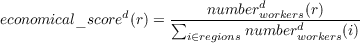
- tactical score: sum of the values of the defender’s armies forces in each
regions, divided by the distance between the region in which each army is
and the region at hand (to a power > 1).
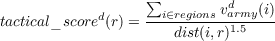 We used a power of 1.5 such that the tactical value of a region in between
two halves of an army, each at distance 2, would be higher than the
tactical value of a region at distance 4 of the full (same) army. For flying
units, dist is the Euclidean distance, while for ground units it takes
pathfinding into account.
We used a power of 1.5 such that the tactical value of a region in between
two halves of an army, each at distance 2, would be higher than the
tactical value of a region at distance 4 of the full (same) army. For flying
units, dist is the Euclidean distance, while for ground units it takes
pathfinding into account.
- ground defense score: the value of the defender’s units which can attack
ground units in region r, divided by the score of ground units of the
attacker in region r.
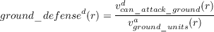
- air defense score: the value of the defender’s units which can attack flying
units in region r, divided by the score of flying units of the attacker in
region r.
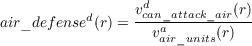
- invisible defense score: the number of the defender’s detectors (units which
can view otherwise invisible units) in region r.

6.3.3 Tech tree
Our model also uses the estimation of the opponent’s tech tree* to know what types
of attacks are possible from them. An introduction to the tech tree is given in
section 4.1.1. The tech tree is the backbone of the strategy: it defines what can
and what cannot be built by the player. The left diagram of Figure 6.3
shows the tech tree of the player after completion of the build order 4.1
in section 4.1.1. The strategic aspect of the tech tree is that it takes time
(between 30 seconds to 2 minutes) to make a building, so tech trees and their
evolutions through time result from a plan and reveal the intention of the
player.
From partial observations, a more complete tech tree can be reconstructed: if an
enemy unit which requires a specific building is seen, one can infer that the whole
tech tree up to this unit’s requirements is available to the opponent’s. Further in
section 7.5, we will show how we took advantage of probabilistic modeling and
learning to infer more about the enemy build tree from partial observation. In this
chapter, we will limit our use of tech trees to be an indicator of what types of attacks
can and cannot be committed.
6.3.4 Attack types
With the discretization of the map into regions and choke-dependent regions, one can
reason about where attacks will happen. The types of the attacks depends on the
units types involved and their use. There may be numerous variations but we
decided to keep the four main types of attacks in the vocabulary of gamers:
- ground attacks, which may use all types of units (and so form the large
majority of attacks). They are constrained by the map topography and by
units collisions so chokes are very important: they are an advantage for
the army with less contact units but enough ranged units or simply more
ranged units, and/or the higher ground.
- air raids, air attacks, which can use only flying units. They are not
constrained by the map, and the mobility of most flying units (except
the largest) allows the player to attack quickly anywhere. Flying units are
most often not cost-effective against ranged ground units, so their first
role is to harass the economy (workers, tech buildings) and fight when in
large numerical superiority (interception, small groups) or against units
which cannot attack air units, all thanks to their mobility and ease of
repositioning.
- invisible (ground) attacks, which can use only a few specific units in
each race (Protoss Dark Templars, Terran Ghosts, Zerg Lurkers). When
detected, this units are not cost-effective. There are two ways to use
invisible attacks: as an all-in as soon as possible (because reaching the
technology required to produce such units is costly and long), before that
the enemy has detection technology. This is a risky strategy but with a
huge payoff (sometimes simply the quick win of the game). The second
way is to try and sneak invisible units behind enemy lines to sap the
opponent’s economy.
- drop attacks, which need a transport unit (Protoss Shuttle, Terran
Dropship, Zerg Overlord with upgrade). Transports give the mobility
of flying units to ground units, with the downsides that units cannot
fire when inside the transport. The usefulness of such attacks comes
from the fact that they are immediately available as soon as the first
transport unit is produced (because the ground units can be produced
before it) and that they do not sacrifice cost-efficiency of most of the
army. The downside is that transports are unarmed and are at the
mercy of interceptions. The goals of such attacks are either to sap the
opponent’s economy (predominantly) or to quickly reinforce an army while
maximizing micro-management of units.
The corresponding goal (orders) are described in section 8.1.2.
6.4 Dataset
6.4.1 Source
We downloaded more than 8000 replays* to keep 7649 uncorrupted, 1v1 replays from
professional gamers leagues and international tournaments of StarCraft, from specialized
websites .
We then ran them using BWAPI
and dumped units’ positions, pathfinding and regions, resources, orders,
vision events, for attacks: types, positions, outcomes. Basically, every
Brood War Application Programmable Interface (BWAPI)* event, plus
attacks, were recorded, the dataset and its source code are freely
available .
The implication of considering only replays of very good player allows us to use this
dataset to learn the behaviors of our bot. Otherwise, particularly regarding the
economy, a simple bot (AI) coupled with a planner can beat the average player, who
does not have a tightly timed build order and/or not the sufficient APM* to
execute.
6.4.2 Information
Table 6.1 shows some metrics about the dataset. In this chapter, we are particularly
interested in the number of attacks. Note that the numbers of attacks for a given race
have to be divided by two in a given non-mirror match-up. So, there are 7072
Protoss attacks in PvP but there are not 70,089 attacks by Protoss in PvT but about
half that.
|
|
|
|
|
|
|
| match-up | PvP | PvT | PvZ | TvT | TvZ | ZvZ |
|
|
|
|
|
|
|
| number of games | 445 | 2408 | 2027 | 461 | 2107 | 199 |
| number of attacks | 7072 | 70089 | 40121 | 16446 | 42175 | 2162 |
| mean attacks/game | 15.89 | 29.11 | 19.79 | 35.67 | 20.02 | 10.86 |
| mean time (frames) / game | 32342 | 37772 | 39137 | 37717 | 35740 | 23898 |
| mean time (minutes) / game | 22.46 | 26.23 | 27.18 | 26.19 | 24.82 | 16.60 |
| mean regions / game | 19.59 | 19.88 | 19.69 | 19.83 | 20.21 | 19.31 |
| mean CDR / game | 41.58 | 41.61 | 41.57 | 41.44 | 42.10 | 40.70 |
| actions issued (game engine) / game | 24584 | 33209 | 31344 | 26998 | 29869 | 21868 |
| mean “BWAPI APM*” (per player) | 547 | 633 | 577 | 515 | 602 | 659 |
| mean ground distance region ↔ region | 2569 | 2608 | 2607 | 2629 | 2604 | 2596 |
| mean ground distance CDR ↔ CDR | 2397 | 2405 | 2411 | 2443 | 2396 | 2401 |
|
|
|
|
|
|
|
| |
Table 6.1: Detailed numbers about our dataset. XvY means race X vs race Y
matches and is an abbreviation of the match-up: PvP stands for Protoss versus
Protoss.
By running the recorded games (replays*) through StarCraft, we were able to
recreate the full state of the game. Time is always expressed in games frames (24
frames per second). We recorded three types of files:
- general data (see appendix B.3): records the players’ names, the map’s
name, and all information about events like creation (along with morph),
destruction, discovery (for one player), change of ownership (special
spell/ability), for each units. It also shows attack events (detected by a
heuristic, see below) and dumps the current economical situation every 25
frames: minerals*, gas*, supply* (count and total: max supply*).
- order data (see appendix B.4): records all the orders which are given to
the units (individually) like move, harvest, attack unit, the orders positions
and their issue time.
- location data (see appendix B.5): records positions of mobile units every
100 frames, and their position in regions and choke-dependent regions
if they changed since last measurement. It also stores ground distances
(pathfinding-wise) matrices between regions and choke-dependent regions
in the header.
From this data, one can recreate most of the state of the game: the map key
characteristics (or load the map separately), the economy of all players, their tech (all
researches and upgrades), all the buildings and units, along with their orders and
their positions.
6.4.3 Attacks
We trigger an attack tracking heuristic when one unit dies and there are at least two
military units around. We then update this attack until it ends, recording every unit
which took part in the fight. We log the position, participating units and fallen units
for each player, the attack type and of course the attacker and the defender.
Algorithm 5
shows how we detect attacks.
6.5 A Bayesian tactical model
6.5.1 Tactical Model
We preferred to map the continuous values from heuristics to a few discrete values to
enable quick complete computations. Another strategy would keep more values and
use Monte-Carlo sampling for computation. We think that discretization is not a
concern because 1) heuristics are simple and biased already 2) we often
reason about imperfect information and this uncertainty tops discretization
fittings.
Variables
With n regions, we have:
- A1:n ∈{true,false}, Ai: attack in region i or not?
- E1:n ∈{no,low,high}, Ei is the discretized economical value of the region
i for the defender. We choose 3 values: no workers in the regions, low: a
small amount of workers (less than half the total) and high: more than
half the total of workers in this region i.
- T1:n ∈ discrete levels, Ti is the tactical value of the region i for the
defender, see above for an explanation of the heuristic. Basically, T is
proportional to the proximity to the defender’s army. In benchmarks,
discretization steps are 0,0.05,0.1,0.2,0.4,0.8 (log2 scale).
- TA1:n ∈ discrete levels, TAi is the tactical value of the region i for the
attacker (as above but for the attacker instead of the defender).
- B1:n ∈ {true,false}, Bi tells if the region belongs (or not) to the
defender. P(Bi = true) = 1 if the defender has a base in region i and
P(Bi = false) = 1 if the attacker has one. Influence zones of the defender
can be measured (with uncertainty) by P(Bi = true) ≥ 0.5 and vice versa.
In fact, when uncertain, P(Bi = true) is proportional to the distance from
i to the closest defender’s base (and vice versa).
- H1:n ∈{ground,air,invisible,drop}, Hi: in predictive mode: how we will
be attacked, in decision-making: how to attack, in region i.
- GD1:n ∈ {no,low,med,high}: ground defense (relative to the attacker
power) in region i, result from a heuristic. no defense if the defender’s
army is ≥ 1∕10th of the attacker’s, low defense above that and under half
the attacker’s army, medium defense above that and under comparable
sizes, high if the defender’s army is bigger than the attacker.
- AD1:n ∈{no,low,med,high}: same for air defense.
- ID1:n ∈{no detector,one detector,several}: invisible defense, equating
to numbers of detectors.
- TT ∈ [∅,building1,building2,building1 ∧ building2,techtrees,…]: all the
possible technological trees for the given race. For instance {pylon,gate}
and {pylon,gate,core} are two different Tech Trees, see chapter 7.
- HP ∈{ground,ground∧air,ground∧invis,ground∧air∧invis,ground∧
drop,ground∧air∧drop,ground∧invis∧drop,ground∧air∧invis∧drop}:
how possible types of attacks, directly mapped from TT information.
This variable serves the purpose of extracting all that we need to know
from TT and thus reducing the complexity of a part of the model from n
mappings from TT to Hi to one mapping from TT to HP and n mapping
from HP to Hi. Without this variable, learning the co-occurrences of
TT and Hi is sparse in the dataset. In prediction, with this variable, we
make use of what we can infer on the opponent’s strategy Synnaeve and
Bessière [2011b], Synnaeve and Bessière [2011], in decision-making, we
know our own possibilities (we know our tech tree as well as the units we
own).
We can consider a more complex version of this tactical model taking soft evidences into
account (variables on which we have a probability distribution), which is presented in
appendix B.2.1.
Decomposition
This decomposition is also shown in Figure 6.4. We can see that we have in fact two
models: one for A1:n and one for H1:n.
Forms and learning
We will explain the forms for a given/fixed i region number:
- P(A) is the prior on the fact that the player attacks in this region, in our
evaluation we set it to nbattles∕(nbattles + nnot battles).
- P(E,T,TA,B|A) is a co-occurrences table of the economical, tactical (both
for the defender and the attacker), belonging scores where an attacks
happen. We just use Laplace’s law of succession (“add one” smoothing)
Jaynes [2003] and count the co-occurrences in the games of the dataset (see
section 6.4), thus almost performing maximum likelihood learning of the
table.

- P(AD,GD,ID|H) is a co-occurrences table of the air, ground, invisible defense
values depending on how the attack happens. As for P(E,T,TA,B|A), we use a
Laplace’s rule of succession learned from the dataset.

- P(H|HP) is the categorical distribution (histogram) on how the attack happens
depending on what is possible. Trivially P(H = ground|HP = ground) = 1.0,
for more complex possibilities we have different smoothed maximum likelihood
multinomial distributions on H values depending on HP.

- P(HP|TT = tt) is a Dirac distribution on the HP = hp which is compatible
with TT = tt. It is the direct mapping of what the tech tree allows as
possible attack types: P(HP = hp|TT) = 1 is a function of TT (all
P(HP≠hp|TT) = 0).
- P(TT): if we are sure of the tech tree (prediction without fog of war, or in
decision-making mode), P(TT = k) = 1 and P(TT≠k) = 0; otherwise, it allows
us to take uncertainty about the opponent’s tech tree and balance P(HP|TT).
We obtain a distribution on what is possible (P(HP)) for the opponent’s attack
types.
There are two approaches to fill up these probability tables, either by observing
games (supervised learning), as we did in the evaluation section, or by acting
(reinforcement learning).
The model is highly modular, and some parts are more important than others.
We can separate three main parts: P(E,T,TA,B|A), P(AD,GD,ID|H) and
P(H|HP). In prediction, P(E,T,TA,B|A) uses the inferred (uncertain) economic
(E), tactical (T) and belonging (B) scores of the opponent while knowing our own
tactical position fully (TA). In decision-making, we know E,T,B (for us) and
estimate TA. In our prediction benchmarks, P(AD,GD,ID|H) has the lesser impact
on the results of the three main parts, either because the uncertainty from
the attacker on AD,GD,ID is too high or because our heuristics are too
simple, though it still contributes positively to the score. In decision-making,
it allows for reinforcement learning to have tuple values for AD,GD,ID
at which to switch attack types. In prediction, P(H|HP) is used to take
P(TT) (coming from strategy prediction [Synnaeve and Bessière, 2011],
chapter 7) into account and constraints H to what is possible. For the use of
P(H|HP)P(HP|TT)P(TT) in decision-making, see the results section (6.6) or the
appendix B.2.1.
Questions
For a given region i, we can ask the probability to attack here,
and the mean by which we should attack, We always sum over estimated, inferred variables, while we know the one we observe
fully. In prediction mode, we sum over TA,B,TT,HP; in decision-making, we sum
over E,T,B,AD,GD,ID (see appendix B.2.1). The complete question that we ask
our model is P(A,H|FullyObserved). The maximum of P(A,H) = P(A) × P(H) may
not be the same as the maximum of P(A) or P(H) take separately. For instance think
of a very important economic zone that is very well defended, it may be the
maximum of P(A), but not once we take P(H) into account. Inversely, some regions
are not defended against anything at all but present little or no interest. Our joint
distribution 6.3 can be rewritten: P(Searched,FullyObserved,Estimated), so we
ask:
The Bayesian program of the model is as follows:
6.6 Results on StarCraft
6.6.1 Learning and posterior analysis
To measure fairly the prediction performance of such a model, we applied
“leave-100-out” cross-validation from our dataset: as we had many games (see
Table 6.2), we set aside 100 games of each match-up for testing (with more than 1
battle per match: rather ≈ 15 battles/match) and train our model on the rest. We
write match-ups XvY with X and Y the first letters of the factions involved
(Protoss, Terran, Zerg). Note that mirror match-ups (PvP, TvT, ZvZ) have
fewer games but twice as many attacks from a given faction (it is twice
the same faction). Learning was performed as explained in section 6.5.1:
for each battle in r we had one observation for: P(er,tr,tar,br|A = true),
and #regions - 1 observations for the i regions which were not attacked:
P(ei≠r,ti≠r,tai≠r,bi≠r|A = false). For each battle of type t we had one observation
for P(ad,gd,id|H = t) and P(H = t|HP = hp). By learning with a Laplace’s law
of succession Jaynes [2003], we allow for unseen event to have a non-zero
probability.
An exhaustive presentation of the learned tables is out of the scope of this
chapter, but we analyzed the posteriors and the learned model concur with human
expertise (e.g. Figures 6.5, 6.6 and 6.7). We looked at the posteriors of:
- P(H) for varying values of GD,AD,ID, by summing on other variables of
the model. Figure 6.5 shows some of the distributions of H in these
conditions:
- (top left plot) We can see that it is far more likely that invisible
(“sneaky”) attacks happen where there is low ground presence, which
concurs with the fact that invisible units are not cost-efficient against
ground units once detected.
- (right plots) Drops at lower values of GD correspond to unexpected
(surprise) drops, because otherwise the defender would have prepared
his army for interception and there would be a high GD (top right
plot). We can also notice than drops are to be preferred either when
it is safe to land (no anti-aircraft defense, bottom right plot) or when
there is a large defense (harassment tactics and/or drops which are
expected by the defender: both right plots).
- (bottom left plot) It is twice more likely to attack a region (by air)
with less than 1/10th of the flying force in anti-aircraft warfare than
to attack a region with up to one half of our force.
Finally, as ground units are more cost efficient than flying units in a static
battle, we see that both P(H = air|AD = 0.0) and P(H = drop|AD = 0.0)
(bottom plots) are much more probable than situations with air defenses: air
raids/attacks are quite risk averse.
- P(H) for varying values of HP, by summing on other variables of the model,
depicted in Figure 6.6. We can see that, in general, there are as many ground
attacks at the sum of other types. The two top graphs show cases in which the
tech of the attacker was very specialized, and, in such cases, the specificity
seems to be used. In particular, the top right graphic may be corresponding to
a “fast Dark Templars rush”.
- P(A) for varying values of T and E, by summing on other variables of the
model, depicted in Figure 6.7. It shows the transition between two types
of encounters: tactics aimed at engaging the enemy army (a higher
T value entails a higher P(A)) and tactics aimed at damaging the
enemy economy (at high E, we look for opportunities to attack with a
small army where T is lower). Higher economical values are strongly
correlated with surprise attacks against low tactical value regions for
the defender (regions which are far from the defender’s army). These
skirmishes almost never happens in open fields (“no eco”: where the
defender has no base) as this would lead to very unbalanced battles (in
terms of army sizes): it would not benefit the smaller party, which
can flee and avoid confrontation, as opposed to when defending their
base.
6.6.2 Prediction performance
Setup
We learned and tested one model for each race and for each match-up. As we want to
predict where (P(A1:n)) and how (P(Hbattle)) the next attack will happen to us, we
used inferred enemy TT (to produce HP) and TA, our scores being fully known: E,
T, B, ID. We consider GD, AD to be fully known even though they depend on the
attacker force, we should have some uncertainty on them, but we tested that they
accounted (being known instead of fully unknown) for 1 to 2% of P(H) accuracy (in
prediction) once HP was known. We should point that pro-gamers scout very
well and so it allows for a highly accurate TT estimation with [Synnaeve
and Bessière, 2011]. The learning phase requires to recreate battle states
(all units’ positions) and count parameters for up to 70,000 battles. Once
that is done, inference is very quick: a look-up in a probability table for
known values and #F look-ups for free variables F on which we sum. We
chose to try and predict the next battle 30 seconds before it happens, 30
seconds being an approximation of the time needed to go from the middle of a
map to all other regions is minimal) to any region by ground, so that the
prediction is useful for the defender (they can position their army). The model
code
(for learning and testing) as well as the datasets (see above) are freely available.
6.6.3 Predictions
Raw results of predictions of positions and types of attacks 30 seconds before they
happen are presented in Table. 6.2: for instance the bold number (38.0) corresponds
to the percentage of good positions (regions) predictions (30 sec before event) which
were ranked 1st in the probabilities on A1:n for Protoss attacks against Terran
(PvT).
- The measures on where corresponds to the percentage of good prediction
and the mean probability for given ranks in P(A1:n) (to give a sense of
the shape of the distribution).
- The measures on how corresponds to the percentage of good predictions
for the most probable P(Hattack) and the ratio of such attack types in the
test set for given attack types. We particularly predict well ground attacks
(trivial in the early game, less in the end game) and, interestingly, Terran
and Zerg drop attacks.
- The where & how row corresponds to the percentage
of good predictions for the maximal probability in the
joint P(A1:n,H1:n): considering only the most probable
attack ,
according to our model, we can predict where and how an attack will
occur in the next 30 seconds ≈ 1/4th of the time.
Mistakes on the type of the attack are high for invisible attacks: while these
tactics can definitely win a game, the counter is strategic (it is to have detectors
technology deployed) more than positional. Also, if the maximum of P(Hbattle) is
wrong, it does not mean than P(Hbattle = good) = 0.0 at all! The result needing
improvements the most is for air tactics, because countering them really is positional,
see our discussion in the conclusion.
We also tried the same experiment 60 seconds before the attack. This gives
even more time for the player to adapt their tactics. Obviously, the tech tree or the
attacker (TT), and thus the possible attack types (HP), are not so different,
nor are the bases possession (belongs, B) and the economy (E). For PvT,
the where top 4 ranks are 35.6, 8.5, 7.7, 7.0% good versus 38.0, 16.3, 8.9,
6.7% 30 seconds before. For the how total precision 60 seconds before is
70.0% vs. 72.4%. where & how maximum probability precision is 19.9% vs.
23%.
Table 6.2: Results summary for multiple metrics at 30 seconds before attack,
including the percentage of the time that it is rightly what happened (%
column). For the where question, we show the four most probable predictions,
the “Pr” column indicates the mean probability of the each bin of the
distribution. For the how question, we show the four types of attacks, their
percentages of correctness in predictions (%) and the ratio of a given attack
type against the total numbers of attacks ( ). The number in bold (38.0) is
read as “38% of the time, the region i with probability of rank 1 in P(Ai) is
the one in which the attack happened 30 seconds later, in the PvT match-up
(predicting Protoss attacks on Terran)”. The associated mean probability for the
first rank of the where measurement is 0.329. The percentage of good predictions
of ground type attacks type in PvT is 98.1%, while ground type attacks, in this
match-up, constitute 54% (ratio of 0.54) of all the attacks. The where & how line
corresponds to the correct predictions of both where and how simultaneously
(as most probables). NA (not available) is in cases for which we do not have
enough observations to conclude sufficient statistics. Remember that attacks
only include fights with at least 3 units involved.
). The number in bold (38.0) is
read as “38% of the time, the region i with probability of rank 1 in P(Ai) is
the one in which the attack happened 30 seconds later, in the PvT match-up
(predicting Protoss attacks on Terran)”. The associated mean probability for the
first rank of the where measurement is 0.329. The percentage of good predictions
of ground type attacks type in PvT is 98.1%, while ground type attacks, in this
match-up, constitute 54% (ratio of 0.54) of all the attacks. The where & how line
corresponds to the correct predictions of both where and how simultaneously
(as most probables). NA (not available) is in cases for which we do not have
enough observations to conclude sufficient statistics. Remember that attacks
only include fights with at least 3 units involved.
|
|
|
|
|
|
|
|
|
|
|
|
|
|
|
|
|
|
|
|
%: good predictions | Protoss | Terran | Zerg
|
Pr=mean probability | P | T | Z | P | T | Z | P | T | Z
|
|
|
|
|
|
|
|
|
|
|
|
|
|
|
|
|
|
|
|
|
| total # games | 445 | 2408 | 2027 | 2408 | 461 | 2107 | 2027 | 2107 | 199
|
|
|
|
|
|
|
|
|
|
|
|
|
|
|
|
|
|
|
|
|
| measure | rank | % | Pr | % | Pr | % | Pr | % | Pr | % | Pr | % | Pr | % | Pr | % | Pr | % | Pr |
|
|
|
|
|
|
|
|
|
|
|
|
|
|
|
|
|
|
|
|
| | 1 | 40.9 | .334 | 38.0 | .329 | 34.5 | .304 | 35.3 | .299 | 34.4 | .295 | 39.0 | 0.358 | 32.8 | .31 | 39.8 | .331 | 37.2 | .324 |
|
where
| 2 | 14.6 | .157 | 16.3 | .149 | 13.0 | .152 | 14.3 | .148 | 14.7 | .147 | 17.8 | .174 | 15.4 | .166 | 16.6 | .148 | 16.9 | .157 |
| | 3 | 7.8 | .089 | 8.9 | .085 | 6.9 | .092 | 9.8 | .09 | 8.4 | .087 | 10.0 | .096 | 11.3 | .099 | 7.6 | .084 | 10.7 | .100 |
| | 4 | 7.6 | .062 | 6.7 | .059 | 7.9 | .064 | 8.6 | .071 | 6.9 | .063 | 7.0 | .062 | 8.9 | .07 | 7.7 | .064 | 8.6 | .07 |
|
|
|
|
|
|
|
|
|
|
|
|
|
|
|
|
|
|
|
|
| measure | type | % |  | % |  | % |  | % |  | % |  | % |  | % |  | % |  | % |  |
|
|
|
|
|
|
|
|
|
|
|
|
|
|
|
|
|
|
|
|
| | G | 97.5 | 0.61 | 98.1 | 0.54 | 98.4 | 0.58 | 100 | 0.85 | 99.9 | 0.66 | 76.7 | 0.32 | 86.6 | 0.40 | 99.8 | 0.84 | 67.2 | 0.34 |
|
how
| A | 44.4 | 0.05 | 34.5 | 0.16 | 46.8 | 0.19 | 40 | 0.008 | 13.3 | 0.09 | 47.1 | 0.19 | 14.2 | 0.10 | 15.8 | 0.03 | 74.2 | 0.33 |
| | I | 22.7 | 0.14 | 49.6 | 0.13 | 12.9 | 0.13 | NA | NA | NA | NA | 36.8 | 0.15 | 32.6 | 0.15 | NA | NA | NA | NA |
| | D | 55.9 | 0.20 | 42.2 | 0.17 | 45.2 | 0.10 | 93.5 | 0.13 | 86 | 0.24 | 62.8 | 0.34 | 67.7 | 0.35 | 81.4 | 0.13 | 63.6 | 0.32 |
| total | 76.3 | 1.0 | 72.4 | 1.0 | 71.9 | 1.0 | 98.4 | 1.0 | 88.5 | 1.0 | 60.4 | 1.0 | 64.6 | 1.0 | 94.7 | 1.0 | 67.6 | 1.0 |
|
|
|
|
|
|
|
|
|
|
|
|
|
|
|
|
|
|
|
|
| where & how (%) | 32.8 | 23 | 23.8 | 27.1 | 23.6 | 30.2 | 23.3 | 30.9 | 26.4
|
|
|
|
|
|
|
|
|
|
|
|
|
|
|
|
|
|
|
|
|
| |
6.6.4 Error analysis
Distance
When we are mistaken, the mean ground distance (pathfinding wise) of the most
probable predicted region to the good one (where the attack happens) is 1223 pixels
(38 build tiles, or 2 screens in StarCraft’s resolution). To put things in perspective,
the tournament maps are mostly between 128 × 128 and 192 × 192 build tiles, and
the biggest maps are of 256 × 256 build tiles.
More interesting is to look at the mean ground distance (see Tables 6.1 and 6.8)
between two regions:
We can see that the most probable predicted region for the attack is not as far of
as if it were random.
Towards a baseline heuristic
The mean number of regions by map is 19, so a random where (attack destination)
picking policy would have a correctness of 1/19 (5.23%). For choke-centered regions,
the numbers of good where predictions are lower (between 24% and 32% correct for
the most probable) but the mean number of regions by map is 42. For where & how,
a random policy would have a precision of 1/(19*4), and even a random policy taking
the high frequency of ground attacks into account would at most be ≈ 1/(19*2)
correct.
For the location only (where question), we also counted the mean number of
different regions which were attacked in a given game (between 3.97 and 4.86 for
regions, depending on the match-up, and between 5.13 and 6.23 for choke-dependent
regions). The ratio over these means would give the prediction rate we could
expect from a baseline heuristic based solely on the location data: a heuristic
which knows totally in which regions we can get attacked and then randomly
select in them. These are attacks that actually happened, so the number of
regions a player have to be worried about is at least this one (or more, for
regions which were not attacked during a game but were potential targets).
This baseline heuristic would yield (depending on the match-up) prediction
rates between 20.5 and 25.2% for regions, versus our 32.8 to 40.9%, and
between 16.1% and 19.5% for choke-dependent regions, versus our 24% to
32%.
Note that our current model consider a uniform prior on regions (no bias
towards past battlefields) and that we do not incorporate any derivative of the
armies’ movements. There is no player modeling at all: learning and fitting the
mean player’s tactics is not optimal, so we should specialize the probability
tables for each player. Also, we use all types of battles in our training and
testing. Short experiments showed that if we used only attacks on bases, the
probability of good where predictions for the maximum of P(A1:n) goes above
50% (which is not a surprise, there are far less bases than regions in which
attacks happen). To conclude on tactics positions prediction: if we sum the 2
most probable regions for the attack, we are right at least half the time; if
we sum the 4 most probable (for our robotic player, it means it prepares
against attacks in 4 regions as opposed to 19), we are right ≈ 70% of the
time.
6.6.5 In-game decision-making
In a StarCraft game, our bot has to make decisions about where and how to
attack or defend, it does so by reasoning about opponent’s tactics, bases, its
priors, and under strategic constraints (Fig. 6). Once a decision is taken,
the output of the tactical model is an offensive or defensive (typed) goal
(see sections 6.3.4 and 8.1.2). The spawned goal then autonomously sets
objectives for Bayesian units Synnaeve and Bessière [2011a], sometimes
procedurally creating intermediate objectives or canceling itself in the worst
cases.
There is no direct way of evaluating decision-making without involving at least
micro-management and others parts of the bot. Regardless, we will explain how the
decision-making process works.
We can use this model to spawn both offensive and defensive goals, either by
taking the most probable attacks/threats, or by sampling in the answer to the
question, or by taking into account the risk of the different plausible attacks
weighted by their probabilities:
- defensive goals (we are the defender, the opponent is the attacker):
- location: P(A1:n)
- type: what counters P(H1:n), what is available close to the most
probable(s) P(A1:n)
- total knowledge: we know fully our army positioning T1:n = t1:n, our
economy E1:n = e1:n, if and where we have detectors ID1:n = id1:n
- partial knowledge: from partial observations, the positioning of the
opponent’s army P(TA1:n), the belonging of regions P(B1:n). We
also infer their tech tree* P(TT) with [Synnaeve and Bessière, 2011]
presented in section 7.5. Note also that, even though we know our
defenses, P(GD1:n) and P(AD1:n) are dependent on the attackers
army: with a gross estimation on the opponent’s forces (from what
we have seen and their tech tree for instance), we can consider that
we know it fully or not. Most often, we have only “soft evidences”
on this variables, which means that we have a distribution on the
variable values. By abusing the notation, we will write P(V ar) for
a variable on which we have a distribution. See appendix B.2.1 for
how to take it into account with coherence variables.
- question:
The question may give back the best tactical interests of the opponent,
taking into account partial observations, their strengths and our
weaknesses. From here we can anticipate and spawn the right defense goals
(put the adequate units at the right place, and even build defensive
structures).
- offensive goals (we are the attacker, the opponent is the defender):
- location: P(A1:n)
- type: P(H1:n)
- total knowledge: we fully know what attack types are possible
HP1:n = hp1:n (our units available, we also know our tech tree
TT = tt but that is useless here), along with our military positions
TA1:n = ta1:n.
- partial knowledge: from partial (potentially outdated) observations,
we have information about E1:n, T1:n, B1:n, ID1:n, GD1:n, AD1:n.
We still abuse the notation with P(V ar) for a variable V ar on which
we only have a distribution (“soft evidence”). See appendix B.2.1 for
how to take it into account with coherence variables.
- question:
The question may give back a couple (i,Hi) more probable than the most
probables P(Ai) and P(Hj) taken separately. For instance in the case of
an heavily defended main base and a small unprotected expansion: the
main base is ranked first economically and possibly tactically, but it may
be too hard to attack, while the unprotected (against a given attack type
is enough) expand is a smaller victory but surer victory. Figure 6.9
displays the mean P(A,H) for Terran (in TvZ) attacks decision-making
for the most 32 probable type/region tactical couples. It is in
this kind of landscape (though more steep because Fig. 6.9 is a
mean) that we sample (or pick the most probable couple) to take a
decision.
Finally, we can steer our technological growth towards the opponent’s weaknesses.
A question that we can ask our model (at time t) is P(TT), or, in two parts: we first
find i,hi which maximize P(A1:n,H1:n) at time t + 1, and then ask a more
directive:
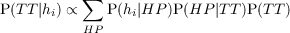 so
that it gives us a distribution on the tech trees (TT) needed to be able to perform
the wanted attack type. To take a decision on our technology direction, we can
consider the distances between our current ttt and all the probable values of
TTt+1.
so
that it gives us a distribution on the tech trees (TT) needed to be able to perform
the wanted attack type. To take a decision on our technology direction, we can
consider the distances between our current ttt and all the probable values of
TTt+1.
6.7 Discussion
6.7.1 In-game learning
The prior on A can be tailored to the opponent (P(A|opponent)). In a given match, it
should be initialized to uniform and progressively learn the preferred attack regions
of the opponent for better predictions. We can also penalize or reward ourselves and
learn the regions in which our attacks fail or succeed for decision-making. Both these
can easily be done with some form of weighted counting (“add-n smoothing”) or even
Laplace’s rule of succession.
In match situation against a given opponent, for inputs that we can unequivocally
attribute to their intention (style and general strategy), we can also refine the
probability tables of P(E,T,TA,B|A,opponent), P(AD,GD,ID|H,opponent)
and P(H|HP,opponent) (with Laplace’s rule of succession). For instance,
we can refine ∑
E,T,TAP(E,T,TA,B|A,opponent) corresponding to their
aggressiveness (aggro) or our successes and failures. Indeed, if we sum over E, T
and TA, we consider the inclination of our opponent to venture into enemy
territory or the interest that we have to do so by counting our successes with
aggressive or defensive parameters. By refining P(H|HP,opponent), we are
learning the opponent’s inclination for particular types of tactics according to
what is available to them, or for us the effectiveness of our attack types
choices.
6.7.2 Possible improvements
There are several main research directions for possible improvements:
- improving the underlying heuristics: the heuristics presented here are quite
simple but they may be changed, and even removed or added, for another RTS
or FPS, or for more performance. In particular, our “defense against invisible”
heuristic could take detector positioning/coverage into account. Our
heuristic on tactical values can also be reworked to take terrain tactical
values into account (chokes and elevation in StarCraft). We now detail
two particular improvements which could increase the performance
significantly:
- To estimate T1:n (tactical value of the defender) when we attack,
or TA1:n (tactical values of the attacker) when we defend, is
the most tricky of all because it may be changing fast. For that
we use a units filter which just decays probability mass of seen
units. An improvement would be to use a particle filter Weber
et al. [2011], additionally with a learned motion model, or a filtering
model adapted to (and taking advantage of) regions as presented in
section 8.1.5.
- By looking at Table 6.2, we can see that our consistently bad
prediction across types is for air attacks. It is an attack type for which
is particularly important to predict to have ranged units (which can
attack flying units) to defend, and because the positioning is so quick
(air units are more mobile). Perhaps we did not have enough data, as
our model fares well in ZvZ for which we have much more air attacks,
but they may also be more stereotyped. Clearly, our heuristics are
missing information about air defense positioning and coverage of
the territory (this is a downside of region discretization). Air raids
work by trying to exploit fine weaknesses in static defense, and they
are not restrained (as ground attacks) to pass through concentrating
chokes.
- improving the dynamic of the model: there is room to improve the dynamics of
the model: considering the prior probabilities to attack in regions given past
attacks and/or considering evolutions of the T,TA,B,E values (derivatives) in
time.
- The discretization that we used may show its limits, though if we want to use
continuous values, we need to setup a more complicated learning and inference
process (Monte-Carlo Markov chain (MCMC)* sampling).
- improving the model itself: finally, one of the strongest assumptions (which is a
drawback particularly for prediction) of our model is that the attacking player
is always considered to attack in this most probable regions. While this
would be true if the model was complete (with finer army positions
inputs and a model of what the player thinks), we believe such an
assumption of completeness is far fetched. Instead we should express that
incompleteness in the model itself and have a “player decision” variable
D ~ Multinomial(P(A1:n,H1:n),player).
Finally, our approach is not exclusive to most of the techniques presented above,
and it could be interesting to combine it with Monte-Carlo planning, as Chung
et al. [2005] did for capture-the-flag tactics in Open RTS. Also, UCT* is a
Monte-Carlo planning algorithm allowing to build a sparse tree over the state tree
(edges are actions, nodes are states) which had excellent results in Go [Gelly and
Wang, 2006, Gelly et al., 2012]. Balla and Fern [2009] showed that UCT could be
used in an RTS game (with multiple simultaneous actions) to generate tactical plans.
Another track (instead of UCT) would be to use metareasoning for MCTS* [Hay and
Russell, 2011], which would incorporate domain knowledge and/or hyper-parameters
(aggressiveness...).
6.7.3 Conclusion
We have presented a Bayesian tactical model for RTS AI, which allows both for
opposing tactics prediction and autonomous tactical decision-making. Being a
probabilistic model, it deals with uncertainty easily, and its design allows easy
integration into multi-granularity (multi-scale) AI systems as needed in RTS AI. The
advantages are that 1) learning will adapt the model output to its biased heuristic
inputs 2) the updating process is the same for offline and online (in-game) learning.
Without any temporal dynamics, the position prediction is above a baseline heuristic
([32.8-40.9%] vs [20.5-25.2%]). Moreover, its exact prediction rate of the joint
position and tactical type is in [23-32.8]% (depending on the match-up), and
considering the 4 most probable regions it goes up to ≈ 70%. More importantly, it
allows for tactical decision-making under (technological) constraints and (state)
uncertainty. It can be used in production thanks to its low CPU and memory
footprint.
Chapter 7
Strategy
Strategy without tactics is the slowest route to victory. Tactics without
strategy is the noise before defeat.
All men can see these tactics whereby I conquer, but what none can see is
the strategy out of which victory is evolved.
What is of supreme importance in war is to attack the enemy’s
strategy.
Sun Tzu (The Art of War, 476-221 BC)
|
WE present our solutions to some of the problems raised at the strategic level.
The main idea is to reduce the complexity encoding all possible variations of
strategies to a few strong indicators: the build tree* (closely related to the tech tree*)
and canonical army compositions. We start by explaining what we consider
that belongs to strategic thinking, and related work. We then describe the
information that we will use and the decisions that can be taken. As we
try and abstract early game strategies to “openings” (as in Chess), we will
present how we labeled a dataset of games with openings. Then, we present
the Bayesian model for build tree prediction (from partial observations),
followed by its augmented version able to predict the opponent’s opening.
Both models were evaluated in prediction dataset of skilled players. Finally
we explain our work on army composition adaptation (to the opponent’s
army).
Build trees estimation was published at the Annual Conference on Artificial
Intelligence and Interactive Digital Entertainment (AAAI AIIDE) 2011 in Palo Alto
[Synnaeve and Bessière, 2011] and openings prediction was published at
Computational Intelligence in Games (IEEE CIG) 2011 in Seoul [Synnaeve and
Bessière, 2011b].
- Problem: take the winning strategy in the absolute (knowing everything:
complete observations, players intentions, effects of each possible actions).
- Problem that we solve: take the winning strategy (in average) knowing
what we saw from the opponent and our model of the game.
- Type: prediction is a problem of inference or plan recognition from
incomplete informations; adaptation given what we know is a problem of
planning under constraints.
- Complexity: simple StarCraft decision problems are NP-hard
[Viglietta, 2012]. We would argue that basic StarCraft strategy
with full information (remember that StarCraft is partially
observable) is mappable to the Generalized Geography
problem
and thus is PSPACE-hard [Lichtenstein and Sipser, 1978], Chess
[Fraenkel and Lichtenstein, 1981] and Go (with Japanese ko rules) are
EXPTIME-complete [Robson, 1983]. Our solutions are real-time on a
laptop.
7.1 What is strategy?
As it is an abstract concept, what constitutes strategy is hard to grasp. The
definition that we use for strategy is a combination of aggressiveness and
“where do we put the cursor/pointer/slider between economy, technology and
military production?”. It is very much related to where we put our resources:
- If we prioritize economy, on a short term basis our army strength
(numbers) may suffer, but on the longer term we will be able to produce
more, or produce equally and still expand our economy or technology in
parallel. Also, keep in mind that resources depletes mineral deposits/gas
geysers can be exhausted/drained.
- If we prioritize technology, on a short term basis our army strength may
suffer, on the longer term it can strive with powerful units or units which
are adapted to the enemy’s.
- If we prioritize military production, on a short term basis our army
strength will strive, but we will not be able to adapt our army composition
to new unit types nor increase our production throughput.
Strategy is a question of balance between these three axis, and of knowing when we can
attack and when we should stay in defense. Being aggressive is best when we have a
military advantage (in numbers or technology) over the opponent. Advantages are
gained by investments in these axis, and capitalizing on them when we max out our
returns (comparatively to the opponent’s).
The other aspect of strategy is to decide what to do with these resources. This is
the part that we studied the most, and the decision-making questions are:
- Where do we expand? (We deal with this question by an ad-hoc solution.)
- Which tech path do we open? Which tech tree do we want to span in a
few minutes? We have to follow a tech tree that enables us to perform the
tactics and long term strategy that we want to do, but we also have to
adapt to whatever the opponent is doing.
- Which unit types, and in which ratios, do we want in our army? We have
a choice in units that we can build, they have costs, we have to decide a
production plan, knowing the possible evolutions of our tech tree and our
possible future production possibilities and capabilities.
In the following, we studied the estimation of the opponent’s strategy in
terms of tech trees* (build trees*), abstracted (labeled) opening* (early
strategy), army composition, and how we should adapt our own strategy to
it.
7.2 Related work
There are precedent works of Bayesian plan recognition [Charniak and Goldman, 1993],
even in games with [Albrecht et al., 1998] using dynamic Bayesian networks to
recognize a user’s plan in a multi-player dungeon adventure. Commercial RTS games
most commonly use FSM* [Houlette and Fu, 2003] to encode strategies and their
transitions.
There are related works in the domains of opponent modeling [Hsieh and
Sun, 2008, Schadd et al., 2007, Kabanza et al., 2010]. The main methods used to
these ends are case-based reasoning (CBR) and planning or plan recognition
[Aha et al., 2005, Ontañón et al., 2008, Ontañón et al., 2007b, Hoang
et al., 2005, Ramírez and Geffner, 2009].
Aha et al. [2005] used CBR* to perform dynamic plan retrieval extracted from
domain knowledge in Wargus (Warcraft II open source clone). Ontañón
et al. [2008] base their real-time case-based planning (CBP) system on a plan
dependency graph which is learned from human demonstration in Wargus. In
[Ontañón et al., 2007b, Mishra et al., 2008b], they use CBR and expert
demonstrations on Wargus. They improve the speed of CPB by using a
decision tree to select relevant features. Hsieh and Sun [2008] based their work
on [Aha et al., 2005] and used StarCraft replays to construct states and
building sequences. Strategies are choices of building construction order in their
model.
Schadd et al. [2007] describe opponent modeling through hierarchically
structured models of the opponent’s behavior and they applied their work to the
Spring RTS game (Total Annihilation open source clone). Hoang et al. [2005] use
hierarchical task networks (HTN*) to model strategies in a first person shooter with
the goal to use HTN planners. Kabanza et al. [2010] improve the probabilistic
hostile agent task tracker (PHATT [Geib and Goldman, 2009], a simulated HMM*
for plan recognition) by encoding strategies as HTN.
Weber and Mateas [2009] presented “a data mining approach to strategy
prediction” and performed supervised learning (from buildings features) on labeled
StarCraft replays. In this chapter, for openings prediction, we worked with the same
dataset as they did, using their openings labels and comparing it to our own labeling
method.
Dereszynski et al. [2011] presented their work at the same conference that we
presented [Synnaeve and Bessière, 2011]. They used an HMM which states are
extracted from (unsupervised) maximum likelihood on the dataset. The HMM
parameters are learned from unit counts (both buildings and military units) every 30
seconds and Viterbi inference is used to predict the most likely next states from
partial observations.
Jónsson [2012] augmented the C4.5 decision tree [Quinlan, 1993] and nearest
neighbour with generalized examplars [Martin, 1995], also used by Weber and
Mateas [2009], with a Bayesian network on the buildings (build tree*). Their results
confirm ours: the predictive power is strictly better and the resistance to
noise far greater than without encoding probabilistic estimations of the build
tree*.
7.3 Perception and interaction
7.3.1 Buildings
From last chapter (section 6.3.3), we recall that the tech tree* is a directed acyclic
graph which contains the whole technological (buildings and upgrades) development
of a player. Also, each unit and building has a sight range that provides the player
with a view of the map. Parts of the map not in the sight range of the player’s units
are under fog of war and the player ignores what is and happens there. We also
recall the notion of build order*: the timings at which the first buildings are
constructed.
In this chapter, we will use build trees* as a proxy for estimating some of
the strategy. A build tree is a little different than the tech tree*: it is the
tech tree without upgrades and researches (only buildings) and augmented
of some duplications of buildings. For instance, {Pylon ∧ Gateway} and
{Pylon∧Gateway,Gateway2} gives the same tech tree but we consider that they are
two different build trees. Indeed, the second Gateway gives some units producing
power to the player (it allows for producing two Gateway units at ones). Very early
in the game, it also shows investment in production and the strategy is less likely to
be focused on quick opening of technology paths/upgrades. We have chosen how
many different versions of a given building type to put in the build trees (as shown in
Table 7.2), so it is a little more arbitrary than the tech trees. Note that
when we know the build tree, we have a very strong conditioning on the tech
tree.
7.3.2 Openings
In RTS games jargon, an opening* denotes the same thing than in Chess: an early
game plan for which the player has to make choices. In Chess because one can not
move many pieces at once (each turn), in RTS games because during the
development phase, one is economically limited and has to choose between economic
and military priorities and can not open several tech paths at once. A rush* is an
aggressive attack “as soon as possible”, the goal is to use an advantage of surprise
and/or number of units to weaken a developing opponent. A push (also timing push
or timing attack) is a solid and constructed attack that aims at striking when the
opponent is weaker: either because we reached a wanted army composition and/or
because we know the opponent is expanding or “teching”. The opening* is also (often)
strongly tied to the first military (tactical) moves that will be performed. It
corresponds to the 5 (early rushes) to 15 minutes (advanced technology / late push)
timespan.
Players have to find out what opening their opponents are doing to be able to
effectively deal with the strategy (army composition) and tactics (military moves:
where and when) thrown at them. For that, players scout each other and reason
about the incomplete information they can bring together about army and buildings
composition. This chapter presents a probabilistic model able to predict the opening*
of the enemy that is used in a StarCraft AI competition entry bot. Instead of
hard-coding strategies or even considering plans as a whole, we consider
the long term evolution of our tech tree* and the evolution of our army
composition separately (but steering and constraining each others), as shown in
Figure 7.1. With this model, our bot asks “what units should I produce?”
(assessing the whole situation), being able to revise and adapt its production
plans.
Later in the game, as the possibilities of strategies “diverge” (as in Chess), there
are no longer fixed foundations/terms that we can speak of as for openings. Instead,
what is interesting is to know the technologies available to the enemy as well as have
a sense of the composition of their army. The players have to adapt to each
other’s technologies and armies compositions either to be able to defend or to
attack. Some units are more cost-efficient than others against particular
compositions. Some combinations of units play well with each others (for
instance biological units with “medics” or a good ratio of strong contact units
backed with fragile ranged or artillery units). Finally, some units can be game
changing by themselves like cloaking units, detectors, massive area of effects
units...
7.3.3 Military units
Strategy is not limited to technology state, openings and timings. The player must
also take strategic decisions about the army composition. While some special tactics
(drops, air raids, invisible attacks) require some specific units, these does not
constitute the bulk of the army, at least not after the first stages of the game (≈ 10
minutes).
The different attack types and “armor” (size) types of units make it so that
pairing units against each others is like a soft rock-paper-scissors (shi-fu-mi). But
there is more to army composition than playing rock-paper-scissors with anticipation
(units take time to be produced) and partial information: some units combine well
with each others. The simplest example of combinations are ranged units and contact
units which can be very weak (lots of weaknesses) taken separately, but they form an
efficient army when combined. There are also units which empower others
through abilities, or units with very strong defensive or offensive abilities with
which one unit can change the course of a battle. As stated before, these
different units need different parts of the tech tree to be available and they
have different resources costs. All things considered, deciding which units to
produce is dependent on the opponent’s army, the requirements of the planned
tactics, the resources and the current (and future) technology available to the
player.
7.4 Replays labeling
A replay* contains all the actions of each players during a game. We used a dataset
of replays to see when the players build which buildings (see Table B.1 in appendix
for an example of the buildings constructions actions). We attributed a label for each
player for each game which notes the players opening*.
7.4.1 Dataset
We used Weber and Mateas [Weber and Mateas, 2009] dataset of labeled replays. It
is composed of 8806 StarCraft: Broodwar game logs, the details are given in
Table 7.1. A match-up* is a set of the two opponents races: Protoss versus Terran
(PvT) is a match-up, Protoss versus Zerg (PvZ) is another one. They are
distinguished because strategies distribution are very different across match-ups
(see Tables 7.1 and 7.3). Weber and Mateas used logic rules on building
sequences to put their labels, concerning only tier 2 strategies (no tier 1
rushes).
|
|
|
|
|
|
|
|
|
|
|
|
| opening | PvP | PvT | PvZ | opening | TvP | TvT | TvZ | opening | ZvP | ZvT | ZvZ |
|
|
|
|
|
|
|
|
|
|
|
|
| FastLegs | 4 | 17 | 108 | Bio | 144 | 41 | 911 | Lurker | 33 | 184 | 1 |
| FastExpand | 119 | 350 | 465 | Unknown | 66 | 33 | 119 | Unknown | 159 | 164 | 212 |
| ReaverDrop | 51 | 135 | 31 | Standard | 226 | 1 | 9 | HydraRush | 48 | 13 | 9 |
| FastObs | 145 | 360 | 9 | SiegeExpand | 255 | 49 | 7 | Standard | 40 | 80 | 1 |
| Unknown | 121 | 87 | 124 | VultureHarass | 134 | 226 | 5 | TwoHatchMuta | 76 | 191 | 738 |
| Carrier | 2 | 8 | 204 | TwoFactory | 218 | 188 | 24 | HydraMass | 528 | 204 | 14 |
| FastDT | 100 | 182 | 83 | FastDropship | 96 | 90 | 75 | ThreeHatchMuta | 140 | 314 | 35 |
|
|
|
|
|
|
|
|
|
|
|
|
| total | 542 | 1139 | 1024 | total | 1139 | 628 | 1150 | total | 1024 | 1150 | 1010 |
|
|
|
|
|
|
|
|
|
|
|
|
| |
Table 7.1: Weber’s dataset with its labels. XvY means the XvY or YvX
match-up but the openings numbers are presented for X.
7.4.2 Probabilistic labeling
Instead of labeling with rules, we used (positive labeling vs rest) clustering of the
opening’s main features to label the games of each player.
The pitfall of logical/rule-based labeling
Openings are closely related to build orders* (BO) but different BO can lead to the
same opening and some BO are shared by different openings. Particularly, if we do
not take into account the time at which the buildings are constructed, we may have a
wrong opening label too often: if an opening consist in having building C as soon as
possible, it does not matter if we built B-A-C instead of the standard A-B-C
as long as we have built C quickly. That is the kind of case that will be
overlooked by logical labeling. For that reason, we tried to label replays with
the statistical appearance of key features with a semi-supervised method
(see Figure 7.2). Indeed, the purpose of our opening prediction model is
to help our StarCraft playing bot to deal with rushes and special tactics.
This was not the main focus of Weber and Mateas’ labels, which follow
exactly the build tree. So, we used the key components of openings that
we want to be aware of as features for our labeling algorithm as shown in
Table 7.2.
Main features of openings
The selection of the features along with the opening labels is the
supervised part of our labeling method. The knowledge of the
features and openings comes from expert play and the StarCraft
Liquipedia
(a Wikipedia for StarCraft). They are all presented in Table 7.2. For instance, if we
want to find out which replays correspond to the “fast Dark Templar” (DT, Protoss
invisible unit) opening, we put the time at which the first Dark Templar is
constructed as a feature and perform clustering on replays with it. This is
what is needed for our playing bot: to be able to know when he has to fear
“fast DT” opening and build a detector unit quickly to be able to deal with
invisibility.
Table 7.2: Opening/Strategies labels of the replays (Weber’s and ours are not
always corresponding)
|
|
|
|
|
| Race | Weber’s labels | Our labels | Features | Note (what we fear) |
|
|
|
|
|
| Protoss | FastLegs | speedzeal | Legs, GroundWeapons+1 | quick speed+upgrade attack |
| | FastDT | fast_dt | DarkTemplar | invisible units |
| | FastObs | nony | Goon, Range | quick long ranged attack |
| | ReaverDrop | reaver_drop | Reaver, Shuttle | tactical attack zone damages |
| | Carrier | corsair | Corsair | flying units |
| | FastExpand | templar | Storm, Templar | powerful zone attack |
| | | two_gates | 2ndGateway, Gateway, | aggressive rush |
| | | | 1stZealot | |
| | Unknown | unknown | (no clear label) | |
|
|
|
|
|
| Terran | Bio | bio | 3rdBarracks, 2ndBarracks, | aggressive rush |
| | | | Barracks | |
| | TwoFactory | two_facto | 2ndFactory | strong push (long range) |
| | VultureHarass | vultures | Mines, Vulture | aggressive harass, invisible |
| | SiegeExpand | fast_exp | Expansion, Barracks | economical advantage |
| | Standard | | | |
| | FastDropship | drop | DropShip | tactical attack |
| | Unknown | unknown | (no clear label) | |
|
|
|
|
|
| Zerg | TwoHatchMuta | fast_mutas | Mutalisk, Gas | early air raid |
| | ThreeHatchMuta | mutas | 3rdHatch, Mutalisk | massive air raid |
| | HydraRush | hydras | Hydra, HydraSpeed, | quick ranged attack |
| | | | HydraRange | |
| | Standard | (speedlings) | (ZerglingSpeed, Zergling) | (removed, quick attacks/mobility) |
| | HydraMass | | | |
| | Lurker | lurkers | Lurker | invisible and zone damages |
| | Unknown | unknown | (no clear label) | |
|
|
|
|
|
| |
Table 7.3: Openings distributions for Terran in all the match-ups. They are
the result of the clustering-based labeling with selection of one label per replay
and per player. We can see that openings usage is different depending on the
match-up*.
|
|
|
|
|
|
|
| | | vs Protoss | | vs Terran | | vs Zerg |
| Opening | Nb | Percentage | Nb | Percentage | Nb | Percentage |
|
|
|
|
|
|
|
| bio | 62 | 6.2 | 25 | 4.4 | 197 | 22.6 |
| fast_exp | 438 | 43.5 | 377 | 65.4 | 392 | 44.9 |
| two_facto | 240 | 23.8 | 127 | 22.0 | 116 | 13.3 |
| vultures | 122 | 12.1 | 3 | 0.6 | 3 | 0.3 |
| drop | 52 | 5.2 | 10 | 1.7 | 121 | 13.9 |
| unknown | 93 | 9.3 | 34 | 5.9 | 43 | 5.0 |
|
|
|
|
|
|
|
| |
Clustering
For the clustering part, we tried k-means and expectation-maximization (EM*, with
Gaussian mixtures) on Gaussian mixtures with shapes and volumes chosen with a
Bayesian information criterion (BIC*). Best BIC models were almost always the most
agreeing with expert knowledge (15/17 labels), so we kept this method. We used
the R package Mclust [Fraley and Raftery, 2002, 2006] to perform full EM
clustering.
The Gaussian mixture model (GMM*) is as follows:
- Variables:
- Xi∈⟦1…n⟧ the features for the ith replay/game. For instance for the
“fast_expand” opening (Barracks and then direct expanding), we
used the features “time of the first expansion” and “time of the first
Barracks”, as is shown in Figure 7.4, and each data point is an Xi.
- Opi∈⟦1…n⟧ the opening of game i. Instead of doing one clustering with
k possible openings, we did k clusterings of 1 opening vs the rest. So
for us Opi ∈{opening,rest}.
- Decomposition (n data points, i.e. n games):
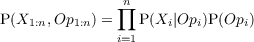
- Forms, for the k openings we have:
- P(Xi|Opi) mixture of (two) Gaussian distributions
- P(Opi) = Bernouilli(pop):
- Identification (EM* with maximum likelihood
estimate ):
Let θ = (μ1:2,σ1:2), initialize θ randomly,
and let L(θ;X) = P(X|θ) = ∏
i=1n ∑
OpiP(Xi|θ,Opi)P(Opi) Iterate until
convergence (of θ):
-
1.
- E-step: Q(θ|θ(t)) = E[log L(θ;x,Op)] =
E[log ∏
i=1n ∑
OpiP(xi|Opi,θ)P(Opi)]
-
2.
- M-step: θ(t+1) = argmaxθQ(θ|θ(t))
- Question (for the ith game):

The σj matrices can define Gaussian distribution of any combinations between:
- volume (of the normal distributions of each mixtures at a given σ value):
equal or variable,
- shape (of the multidimensional normal distributions of each mixtures):
equal or variable,
- orientation: spherical (i.e. no orientation), coordinate axes, equal (any
orientation although the same for all mixtures components) or variable
(any orientation for any component).
A σ with variable volume, variable shape and variable orientation is also called a full
covariance matrix. We chose the combinations with the best (i.e. smallest) BIC*
score. For a given model with n data points, m parameters and L the maximum
likelihood, BIC = -2ln(L) + mln(n).
Labeling, score filtering
The whole process of labeling replays (games) is shown in Figure 7.2. We produce “2
bins clustering” for each set of features (corresponding to each opening), and label
the replays belonging to the cluster with the lower norm of features’ appearances
(that is exactly the purpose of our features). Figures 7.5, 7.4 and 7.6 show the
clusters out of EM with the features of the corresponding openings. We thought of
clustering because there are two cases in which you build a specific military unit or
research a specific upgrade: either it is part of your opening, or it is part of your
longer term game plan or even in reaction to the opponent. So the distribution over
the time at which a feature appears is bimodal, with one (sharp) mode corresponding
to “opening with it” and the other for the rest of the games, as can be seen in
Figure 7.3.
Due to the different time of effect of different openings, some replays are labeled
two or three times with different labels. So, finally, we apply a score filtering to
transform multiple label replays into unique label ones (see Figure 7.2). For that we
choose the openings labels that were happening the earliest (as they are a closer
threat to the bot in a game setup) if and only if they were also the most
probable or at 10% of probability of the most probable label (to exclude
transition boundaries of clusters) for this replay. We find the earliest by
comparing the norms of the clusters means in competition. All replays without a
label or with multiple labels (i.e. which did not had a unique solution in
filtering) after the filtering were labeled as unknown. An example of what is the
final distribution amongst replays’ openings labels is given for the three
Terran match-ups* in Table 7.3. We then used this labeled dataset as well as
Weber and Mateas’ labels in the testing of our Bayesian model for opening
prediction.
7.5 Build tree prediction
The work described in the next two sections can be classified as probabilistic plan
recognition. Strictly speaking, we present model-based machine learning used for
prediction of plans, while our model is not limited to prediction. We performed two
levels of plan recognition, both are learned from the replays: tech tree prediction
(unsupervised, it does not need openings labeling, this section) and opening
prediction (semi-supervised or supervised depending on the labeling method, next
section).
7.5.1 Bayesian model
Variables
- BuildTree: BT ∈{∅,{building1},{building2},{building1∧building2},…}:
all the possible building trees for the given race. For instance {pylon,gate}
and {pylon,gate,core} are two different BuildTrees.
- Observations: Oi∈⟦1…N⟧ ∈{0,1}, Ok is 1∕true if we have seen (observed)
the kth building (it can have been destroyed, it will stay “seen”). Otherwise,
it is 0∕false.
- λ ∈ {0,1}: coherence variable (restraining BuildTree to possible values
with regard to O1:N)
- Time: T ∈⟦1…P⟧, time in the game (1 second resolution).
At first, we generated all the possible (according to the game rules) build trees* (BT
values) of StarCraft, and there are between ≈ 500 and 1600 depending on the race
without even counting buildings duplicates! We observed that a lot of possible
build trees are too absurd to be performed in a competitive match and were
never seen during the learning. So, we restricted BT to have its value in all
the build trees encountered in our replays dataset and we added multiple
instances of the basic unit producing buildings (gateway, barracks), expansions
and supply buildings (depot, pylon, “overlord” as a building), as shown in
Table 7.2. This way, there are 810 build trees for Terran, 346 for Protoss and
261 for Zerg (learned from ≈ 3000 games for each race, see Table 7.1). In
a new game, if we encounter a build tree that we never saw, we are in a
unknown state. Anyway we would not have seen enough data (any at all) during
the learning to conclude anything. We could look at the proximity of the
build tree to other known build trees, see section 7.5.2 and the Discussion
(7.5.3).
Decomposition
The joint distribution of our model is the following:
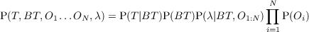 | (7.1) |
This can also be see as a plate diagram in Figure 7.7.
Forms
- P(BT) is the prior distribution on the build trees. As we do not want to
include any bias, we set it to the uniform distribution.
- P(O1:N) is unspecified, we put the uniform distribution (we could use a
prior over the most frequent observations).
- P(λ|BT,O1:N) is a functional Dirac that restricts BT values to the ones than
can co-exist with the observations: A build tree value (bt) is compatible with the observations if it covers them
fully. For instance, BT = {pylon,gate,core} is compatible with ocore = 1 but it
is not compatible with oforge = 1. In other words, buildTree is incompatible
with o1:N iff {o1:N\{o1:N ∧ buildTree}}≠∅.
- P(T|BT = bt) =
 (μbt,σbt2): P(T|BT) are discrete normal distributions (“bell
shapes”). There is one bell shape over T per bt. The parameters of these
discrete Gaussian distributions are learned from the replays.
(μbt,σbt2): P(T|BT) are discrete normal distributions (“bell
shapes”). There is one bell shape over T per bt. The parameters of these
discrete Gaussian distributions are learned from the replays.
Identification (learning)
As we have full observations in the training phase, learning is just counting and
averaging. The learning of the P(T|BT) bell shapes parameters takes into account
the uncertainty of the bt for which we have few observations: the normal distribution
P(T|bt) begins with a high σbt2, and not a strong peak at μbt on the seen T value
and sigma = 0. This accounts for the fact that the first(s) observation(s) may be
outlier(s). This learning process is independent on the order of the stream of
examples, seeing point A and then B or B and then A in the learning phase produces
the same result.
Questions
The question that we will ask in all the benchmarks is:
 | (7.2) |
An example of the evolution of this question with new observations is depicted in
Figure 7.8, in which we can see that build trees (possibly closely related) succeed
each others (normal) until convergence.
Bayesian program
The full Bayesian program is:
7.5.2 Results
All the results presented in this section represents the nine match-ups (races
combinations) in 1 versus 1 (duel) of StarCraft. We worked with a dataset of 8806
replays (≈ 1000 per match-up) of skilled human players (see 7.1) and we
performed cross-validation with 9/10th of the dataset used for learning and
the remaining 1/10th of the dataset used for evaluation. Performance wise,
the learning part (with ≈ 1000 replays) takes around 0.1 second on a 2.8
Ghz Core 2 Duo CPU (and it is serializable). Each inference (question) step
takes around 0.01 second. The memory footprint is around 3Mb on a 64 bits
machine.
Metrics
k is the numbers of buildings ahead that we can accurately predict the build tree of
the opponent at a fixed d. d values are distances between the predicted build tree(s)
and the reality (at fixed k).
The robustness to noise is measured by the distance d to the real build tree
with increasing levels of noise, for k = 0.
The predictive power of our model is measured by the k > 0 next
buildings for which we have “good enough” prediction of future build trees
in:

“Good enough” is measured by a distance d to the actual build
tree of the opponent that we tolerate. We used a set distance:
d(bt1,bt2) = card(bt1Δbt2) = card((bt1 ⋃
bt2)\(bt1 ⋂
bt2)). One less or more building
in the prediction is at a distance of 1 from the actual build tree. The same set of
buildings except for one replacement is at a distance of 2 (that would be 1 is we used
tree edit distance with substitution).
- We call d(best,real) =“best” the distance between the most probable build
tree and the one that actually happened.
- We call d(bt,real)*P(bt)=“mean” the marginalized distance between what
was inferred balanced (variable bt) by the probability of inferences (P(bt)).
Note that this distance is always over the complete build tree, and not only the newly
inferred buildings. This distance metric was counted only after the fourth (4th)
building so that the first buildings would not penalize the prediction metric (the first
building can not be predicted 4 buildings in advance).
For information, the first 4 buildings for a Terran player are more often amongst
his first supply depot, barracks, refinery (gas), and factory or expansion or second
barracks. For Zerg, the first 4 buildings are is first overlord, zergling pool, extractor
(gas), and expansion or lair tech. For Protoss, it can be first pylon, gateway,
assimilator (gas), cybernectics core, and sometimes robotics center, or forge or
expansion.
Table 7.4 shows the full results, the first line has to be interpreted
as “without noise, the average of the following measures are” (columns):
- d for k = 0:
- d(best,real) = 0.535, it means that the average distance from the
most probable (“best”) build tree to the real one is 0.535 building.
- d(bt,real) * P(bt) = 0.870, it means that the average distance
from each value bt of the distribution on BT, weighted by its own
probability (P(bt)), to the real one is 0.87 building.
- k for d = 1:
- best k = 1.193, it means that the average number of buildings ahead
(of their construction) that the model predicts at a fixed maximum
error of 1 (d = 1) for the most probable build tree (“best”) is 1.193
buildings.
- “mean” k = 3.991, it means that the average number
of buildings ahead (of their construction) that the
model predicts at a fixed maximum error 1 (d = 1),
summed for bt in BT value and weighted by P(bt) is
3.991
- idem that the bullet above but k for d = 2 and d = 3.
The second line (“min”) is the minimum across the different match-ups* (as they are
detailed for noise = 10%), the third (“max”) is for the maximum across match-ups,
both still at zero noise. Subsequent sets of lines are for increasing values of noise (i.e.
missing observations).
Predictive power
To test the predictive power of our model, we are interested at looking at how big k
is (how much “time” before we can predict a build tree) at fixed values of d. We used
d = 1,2,3: with d = 1 we have a very strong sense of what the opponent is doing or
will be doing, with d = 3, we may miss one key building or the opponent may have
switched of tech path.
We can see in Table 7.4 that with d = 1 and without noise (first line), our model
predicts in average more than one building in advance (k > 1) what the opponent
will build next if we use only its best prediction. If we marginalize over BT (sum on
BT weighted by P(bt)), we can almost predict four buildings in advance. Of course,
if we accept more error, the predictive power (number of buildings ahead that our
model is capable to predict) increases, up to 6.122 (in average) for d = 3 without
noise.
Table 7.4: Summarization of the main results/metrics, one full results set for
10% noise
|
|
|
|
|
|
|
|
|
|
| | measure | d for k = 0 | k for d = 1 | k for d = 2 | k for d = 3 |
| noise | |
d(best,real) | d(bt,real) * P(bt) | best | “mean” | best | “mean” | best | “mean” |
|
|
|
|
|
|
|
|
|
|
|
0% | average | 0.535 | 0.870 | 1.193 | 3.991 | 2.760 | 5.249 | 3.642 | 6.122 |
| | min | 0.313 | 0.574 | 0.861 | 2.8 | 2.239 | 3.97 | 3.13 | 4.88 |
| | max | 1.051 | 1.296 | 2.176 | 5.334 | 3.681 | 6.683 | 4.496 | 7.334 |
|
|
|
|
|
|
|
|
|
|
|
10% | PvP | 0.397 | 0.646 | 1.061 | 2.795 | 2.204 | 3.877 | 2.897 | 4.693 |
| | PvT | 0.341 | 0.654 | 0.991 | 2.911 | 2.017 | 4.053 | 2.929 | 5.079 |
| | PvZ | 0.516 | 0.910 | 0.882 | 3.361 | 2.276 | 4.489 | 3.053 | 5.308 |
| | TvP | 0.608 | 0.978 | 0.797 | 4.202 | 2.212 | 5.171 | 3.060 | 5.959 |
| | TvT | 1.043 | 1.310 | 0.983 | 4.75 | 3.45 | 5.85 | 3.833 | 6.45 |
| | TvZ | 0.890 | 1.250 | 1.882 | 4.815 | 3.327 | 5.873 | 4.134 | 6.546 |
| | ZvP | 0.521 | 0.933 | 0.89 | 3.82 | 2.48 | 4.93 | 3.16 | 5.54 |
| | ZvT | 0.486 | 0.834 | 0.765 | 3.156 | 2.260 | 4.373 | 3.139 | 5.173 |
| | ZvZ | 0.399 | 0.694 | 0.9 | 2.52 | 2.12 | 3.53 | 2.71 | 4.38 |
| | average | 0.578 | 0.912 | 1.017 | 3.592 | 2.483 | 4.683 | 3.213 | 5.459 |
| | min | 0.341 | 0.646 | 0.765 | 2.52 | 2.017 | 3.53 | 2.71 | 4.38 |
| | max | 1.043 | 1.310 | 1.882 | 4.815 | 3.45 | 5.873 | 4.134 | 6.546 |
|
|
|
|
|
|
|
|
|
|
|
20% | average | 0.610 | 0.949 | 0.900 | 3.263 | 2.256 | 4.213 | 2.866 | 4.873 |
| | min | 0.381 | 0.683 | 0.686 | 2.3 | 1.858 | 3.25 | 2.44 | 3.91 |
| | max | 1.062 | 1.330 | 1.697 | 4.394 | 3.133 | 5.336 | 3.697 | 5.899 |
|
|
|
|
|
|
|
|
|
|
|
30% | average | 0.670 | 1.003 | 0.747 | 2.902 | 2.055 | 3.801 | 2.534 | 4.375 |
| | min | 0.431 | 0.749 | 0.555 | 2.03 | 1.7 | 3 | 2.22 | 3.58 |
| | max | 1.131 | 1.392 | 1.394 | 3.933 | 2.638 | 4.722 | 3.176 | 5.268 |
|
|
|
|
|
|
|
|
|
|
|
40% | aerage | 0.740 | 1.068 | 0.611 | 2.529 | 1.883 | 3.357 | 2.20 | 3.827 |
| | min | 0.488 | 0.820 | 0.44 | 1.65 | 1.535 | 2.61 | 1.94 | 3.09 |
| | max | 1.257 | 1.497 | 1.201 | 3.5 | 2.516 | 4.226 | 2.773 | 4.672 |
|
|
|
|
|
|
|
|
|
|
|
50% | average | 0.816 | 1.145 | 0.493 | 2.078 | 1.696 | 2.860 | 1.972 | 3.242 |
| | min | 0.534 | 0.864 | 0.363 | 1.33 | 1.444 | 2.24 | 1.653 | 2.61 |
| | max | 1.354 | 1.581 | 1 | 2.890 | 2.4 | 3.613 | 2.516 | 3.941 |
|
|
|
|
|
|
|
|
|
|
|
60% | average | 0.925 | 1.232 | 0.400 | 1.738 | 1.531 | 2.449 | 1.724 | 2.732 |
| | min | 0.586 | 0.918 | 0.22 | 1.08 | 1.262 | 1.98 | 1.448 | 2.22 |
| | max | 1.414 | 1.707 | 0.840 | 2.483 | 2 | 3.100 | 2.083 | 3.327 |
|
|
|
|
|
|
|
|
|
|
|
70% | average | 1.038 | 1.314 | 0.277 | 1.291 | 1.342 | 2.039 | 1.470 | 2.270 |
| | min | 0.633 | 0.994 | 0.16 | 0.79 | 1.101 | 1.653 | 1.244 | 1.83 |
| | max | 1.683 | 1.871 | 0.537 | 1.85 | 1.7 | 2.512 | 1.85 | 2.714 |
|
|
|
|
|
|
|
|
|
|
|
80% | average | 1.134 | 1.367 | 0.156 | 0.890 | 1.144 | 1.689 | 1.283 | 1.831 |
| | min | 0.665 | 1.027 | 0.06 | 0.56 | 0.929 | 1.408 | 1.106 | 1.66 |
| | max | 1.876 | 1.999 | 0.333 | 1.216 | 1.4 | 2.033 | 1.5 | 2.176 |
|
|
|
|
|
|
|
|
|
|
| |
Robustness to missing informations (“noise”)
The robustness of our algorithm is measured by the quality of the predictions of the
build trees for k = 0 (reconstruction, estimation) or k > 0 (prediction) with missing
observations in:

The “reconstructive” power (infer what has not been seen) ensues from the
learning of our parameters from real data: even in the set of build trees that are
possible, with regard to the game rules, only a few will be probable at a given time
and/or with some key structures. The fact that we have a distribution on BT allows
us to compare different values bt of BT on the same scale and to use P(BT) (“soft
evidence”) as an input in other models. This “reconstructive” power of our model is
shown in Table 7.4 with d (distance to actual building tree) for increasing noise at
fixed k = 0.
Figure 7.9 displays first (on top) the evolution of the error rate in reconstruction
(distance to actual building) with increasing random noise (from 0% to 80%, no
missing observations to 8 missing observations over 10). We consider that having an
average distance to the actual build tree a little over 1 for 80% missing observations
is a success. This means that our reconstruction of the enemy build tree with a few
rightly timed observations is very accurate. We should ponder that this average
“missed” (unpredicted or wrongly predicted) building can be very important (for
instance if it unlocks game changing technology). We think that this robustness to
noise is due to P(T|BT) being precise with the amount of data that we used, and the
build tree structure.
Secondly, Figure 7.9 displays (at the bottom) the evolution of the predictive
power (number of buildings ahead from the build tree that it can predict)
with the same increase of noise. Predicting 2 building ahead with d = 1
(1 building of tolerance) gives that we predict right (for sure) at least one
building, at that is realized up to almost 50% of noise. In this case, this
“one building ahead” right prediction (with only 50% of the information)
can give us enough time to adapt our strategy (against a game changing
technology).
7.5.3 Possible improvements
We recall that we used the prediction of build trees (or tech trees), as a proxy for the
estimation of an opponent’s technologies and production capabilities.
This work can be extended by having a model for the two players (the bot/AI and
the opponent):
 So
that we could ask this (new) model:
So
that we could ask this (new) model:
 This would allow for simple and dynamic build tree adaptation to the opponent
strategy (dynamic re-planning), by the inference path: That way, one can ask “what build/tech tree should I go for against what I see from
my opponent”, which tacitly seeks the distribution on BTop to break the complexity
of the possible combinations of O1:N. It is possible to not marginalize over BTop, but
consider only the most probable(s) BTop. In this usage, a filter on BTbot (as simple
as P(BTbott|BTbott-1) can and should be added to prevent switching build orders or
strategies too often.
This would allow for simple and dynamic build tree adaptation to the opponent
strategy (dynamic re-planning), by the inference path: That way, one can ask “what build/tech tree should I go for against what I see from
my opponent”, which tacitly seeks the distribution on BTop to break the complexity
of the possible combinations of O1:N. It is possible to not marginalize over BTop, but
consider only the most probable(s) BTop. In this usage, a filter on BTbot (as simple
as P(BTbott|BTbott-1) can and should be added to prevent switching build orders or
strategies too often.
7.6 Openings
7.6.1 Bayesian model
We now build upon the previous build tree* predictor model to predict the
opponent’s strategies (openings) from partial observations.
Variables
As before, we have:
- Build trees:
BT ∈ [∅,building1,building2,building1 ∧ building2,techtrees,…]: all the
possible building trees for the given race. For instance {pylon,gate} and
{pylon,gate,core} are two different BT.
- N Observations: Oi∈⟦1…N⟧ ∈ {0,1}, Ok is 1 (true) if we have seen
(observed) the kth building (it can have been destroyed, it will stay “seen”).
- Coherence variable: λ ∈ {0,1}: coherence variable (restraining BT to
possible values with regard to O⟦1…N⟧)
- Time: T ∈⟦1…P⟧, time in the game (1 second resolution).
Additionally, we have:
- Opening: Opt ∈ [opening1…openingM] take the various opening values
(depending on the race), with opening labels as described in section 7.3.2.
- Last opening: Opt-1 ∈ [opening1…openingM], opening value of the
previous time step (this allows filtering, taking previous inference into
account).
Decomposition
The joint distribution of our model is the following:
This can also be seen as Figure 7.10.
Forms
- P(Opt|Opt-1), we use it as a filter, so that we take into account previous
inferences (compressed). We use a Dirac: This does not prevent our model to switch predictions, it just uses the previous
inference’s posterior P(Opt-1) to average P(Opt).
- P(Opt-1) is copied from one inference to another (mutated from P(Opt)). The
first P(Opt-1) is bootstrapped with the uniform distribution. We could also use
a prior on openings in the given match-up, which is directly shown in
Tables 7.1 and 7.3.
- P(BT|Opt = op) = Categorical(
 ,pop) is learned from the labeled replays.
P(BT|Opt) are M (#{openings}) different histogram over the values of
BT.
,pop) is learned from the labeled replays.
P(BT|Opt) are M (#{openings}) different histogram over the values of
BT.
- P(Oi∈⟦1…N⟧) is unspecified, we put the uniform distribution.
- P(λ|BuildTree,O⟦1…N⟧) is a functional Dirac that restricts BuildTree values to
the ones than can co-exist with the observations. As explained above in the
build tree model.
- P(T|BT = bt,Opt = op) = (μbt,op,σbt,op2): P(T|BT,Opt) are discrete normal
distributions (“bell shapes”). There is one bell shape over T per couple
(opening,buildTree). The parameters of these discrete Gaussian distributions
are learned from the labeled replays.
Identification (learning)
The learning of the P(BT|Opt) histogram is straight forward counting of occurrences
from the labeled replays with “add-one smoothing” (Laplace’s law of succession
[Jaynes, 2003]):
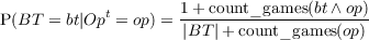
The learning of the P(T|BT,Opt) bell shapes parameters takes into account the
uncertainty of the couples (bt,op) for which we have few observations. This is even
more important as observations may (will) be sparse for some values of Opt, as can
be seen in Figure 7.11. As for the previous, the normal distribution P(T|bt,op)
begins with a high σbt,op2. This accounts for the fact that the first(s) observation(s)
may be outlier(s).
Questions
The question that we will ask in all the benchmarks is:
Note that if we see P(BT,Time) as a plan, asking P(BT|Opt,Time) boils down to
use our “plan recognition” mode as a planning algorithm. This gives us a
distribution on the build trees to follow (build orders) to achieve a given
opening.
Bayesian program
7.6.2 Results
Metrics
For each match-up, we ran cross-validation testing with 9/10th of the dataset used
for learning and the remaining 1/10th of the dataset used for testing. We ran tests
finishing at 5, 10 and 15 minutes to capture all kinds of openings (early to late
ones). To measure the predictive capability of our model, we used 3 metrics:
- the final prediction, which is the opening that is predicted at the end of
the test,
- the online twice (OT), which counts the openings that have emerged as
most probable twice a test (so that their predominance is not due to noise),
- the online once > 3 (OO3), which counts the openings that have emerged
as most probable openings after 3 minutes (so that these predictions are
based on really meaningful information).
After 3 minutes, a Terran player will have built his first supply depot, barracks, refinery
(gas), and at least factory or expansion. A Zerg player would have his first
overlord, zergling pool, extractor (gas) and most of the time his expansion and
lair tech. A Protoss player would have his first pylon, gateway, assimilator
(gas), cybernectics core, and sometimes his robotics center, or forge and
expansion.
Predictive power
Table 7.8 sums up all the prediction probabilities (scores) for the most probable
opening according to our model (compared to the replay label) in all the match-ups
with both labeling of the game logs. The first line should be read as: in the
Protoss vs Protoss (PvP) match-up*, with the rule-based openings labels
(Weber’s labels), the most probable opening* (in the Op values) at 5 minutes
(“final”) is 65% correct. The proportion of times that the most probable
opening twice (“OT”) in the firsts 5 minutes period was the real one (the
game label for this player) is 53%. The proportion of times that the most
probable opening after 3 minutes (“OO3”) and in the firsts 5 minutes periods
was the real one is 0.59%. Then the other columns show the same metrics
for 10 and 15 minutes periods, and then the same with our probabilistic
clustering.
Note that when an opening is mispredicted, the distribution on openings
is often not P(badopening) = 1,P(others) = 0 and that we can extract
some value out of these distributions (see the bot’s strategy adaptation in
chapter 8). Also, we observed that P(Opening = unknown) > P(others)
is often a case of misprediction: our bot uses the next prediction in this
case.
Figure 7.12 shows the evolutions of the distribution P(Opening) during a game
for Weber’s and our labeling or the openings. We can see that in this game, their
build tree* and rule-based labeling (top plot) enabled the model to converge faster
towards FastDropship. With our labeling (bottom plot), the corresponding drop
opening peaked earlier (5th building vs 6th with their labeling) but it was then
eclipsed by two_facto (while staying good second) until later with another key
observation (11th building). This may due to unorthodox timings of the drop
opening, probably because the player was delayed (by a rush, or changed his mind),
and that the two_facto opening has a larger (more robust to delays) support in the
dataset.
Robustness to noise
Figure 7.13 shows the resistance of our model to noise. We randomly removed
some observations (buildings, attributes), from 1 to 15, knowing that for
Protoss and Terran we use 16 buildings observations and 17 for Zerg. We
think that our model copes well with noise because it backtracks unseen
observations: for instance if we have only the core observation, it will work
with build trees containing core that will passively infer unseen pylon and
gate.
Table 7.5: Prediction probabilities for all the match-ups, at 5 minutes, 10
minutes, 15 minutes, both for Weber’s labels and for our labels. The three
metrics are 1) final: what is the most probable at the end of the time equals
compared to the label, 2) OT: (online twice) what was the most probable in
two different inferences during the game compared to the label, 3) OO3 (online
once > 3 minutes) what was the most probable opening after 3 minutes of game
compared to the label.
|
|
|
|
|
|
|
|
|
|
|
|
|
|
|
|
|
|
|
| | | Weber and Mateas’ labels
| Our labels
|
|
|
|
|
|
|
|
|
|
|
|
|
|
|
|
|
|
|
| | 5 minutes | 10 minutes | 15 minutes | 5 minutes | 10 minutes | 15 minutes
|
| match-up | final | OT | OO3 | final | OT | OO3 | final | OT | OO3 | final | OT | OO3 | final | OT | OO3 | final | OT | OO3 |
|
|
|
|
|
|
|
|
|
|
|
|
|
|
|
|
|
|
|
| PvP | 0.65 | 0.53 | 0.59 | 0.69 | 0.69 | 0.71 | 0.65 | 0.67 | 0.73 | 0.78 | 0.74 | 0.68 | 0.83 | 0.83 | 0.83 | 0.85 | 0.83 | 0.83 |
| PvT | 0.75 | 0.64 | 0.71 | 0.78 | 0.86 | 0.83 | 0.81 | 0.88 | 0.84 | 0.62 | 0.69 | 0.69 | 0.62 | 0.73 | 0.72 | 0.6 | 0.79 | 0.76 |
| PvZ | 0.73 | 0.71 | 0.66 | 0.8 | 0.86 | 0.8 | 0.82 | 0.87 | 0.8 | 0.61 | 0.6 | 0.62 | 0.66 | 0.66 | 0.69 | 0.61 | 0.62 | 0.62 |
| TvP | 0.69 | 0.63 | 0.76 | 0.6 | 0.75 | 0.77 | 0.55 | 0.73 | 0.75 | 0.50 | 0.47 | 0.54 | 0.5 | 0.6 | 0.69 | 0.42 | 0.62 | 0.65 |
| TvT | 0.57 | 0.55 | 0.65 | 0.5 | 0.55 | 0.62 | 0.4 | 0.52 | 0.58 | 0.72 | 0.75 | 0.77 | 0.68 | 0.89 | 0.84 | 0.7 | 0.88 | 0.8 |
| TvZ | 0.84 | 0.82 | 0.81 | 0.88 | 0.91 | 0.93 | 0.89 | 0.91 | 0.93 | 0.71 | 0.78 | 0.77 | 0.72 | 0.88 | 0.86 | 0.68 | 0.82 | 0.81 |
| ZvP | 0.63 | 0.59 | 0.64 | 0.87 | 0.82 | 0.89 | 0.85 | 0.83 | 0.87 | 0.39 | 0.56 | 0.52 | 0.35 | 0.6 | 0.57 | 0.41 | 0.61 | 0.62 |
| ZvT | 0.59 | 0.51 | 0.59 | 0.68 | 0.69 | 0.72 | 0.57 | 0.68 | 0.7 | 0.54 | 0.63 | 0.61 | 0.52 | 0.67 | 0.62 | 0.55 | 0.73 | 0.66 |
| ZvZ | 0.69 | 0.64 | 0.67 | 0.73 | 0.74 | 0.77 | 0.7 | 0.73 | 0.73 | 0.83 | 0.85 | 0.85 | 0.81 | 0.89 | 0.94 | 0.81 | 0.88 | 0.94 |
|
|
|
|
|
|
|
|
|
|
|
|
|
|
|
|
|
|
|
| overall | 0.68 | 0.62 | 0.68 | 0.73 | 0.76 | 0.78 | 0.69 | 0.76 | 0.77 | 0.63 | 0.67 | 0.67 | 0.63 | 0.75 | 0.75 | 0.63 | 0.75 | 0.74 |
|
|
|
|
|
|
|
|
|
|
|
|
|
|
|
|
|
|
|
| |
Computational performances
The first iteration of this model was not making use of the structure imposed by the
game in the form of “possible build trees” and was at best very slow, at worst
intractable without sampling. With the model presented here, the performances
are ready for production as shown in Table 7.6. The memory footprint is
around 3.5Mb on a 64bits machine. Learning computation time is linear in
the number of games logs events (O(N) with N observations), which are
bounded, so it is linear in the number of game logs. It can be serialized
and done only once when the dataset changes. The prediction computation
corresponds to the sum in the question (III.B.5) and so its computational
complexity is in O(N ⋅ M) with N build trees and M possible observations, as
M << N, we can consider it linear in the number of build trees (values of
BT).
Table 7.6: Extremes of computation time values (in seconds, Core 2 Duo
2.8Ghz)
|
|
|
|
|
| Race | Nb Games | Learning time | Inference μ | Inference σ2 |
|
|
|
|
|
| T (max) | 1036 | 0.197844 | 0.0360234 | 0.00892601 |
| T (Terran) | 567 | 0.110019 | 0.030129 | 0.00738386 |
| P (Protoss) | 1021 | 0.13513 | 0.0164457 | 0.00370478 |
| P (Protoss) | 542 | 0.056275 | 0.00940027 | 0.00188217 |
| Z (Zerg) | 1028 | 0.143851 | 0.0150968 | 0.00334057 |
| Z (Zerg) | 896 | 0.089014 | 0.00796715 | 0.00123551 |
|
|
|
|
|
| |
Strengths and weaknesses of StarCraft openings
We also proceeded to analyze the strengths and weaknesses of openings against each
others. For that, we labeled the dataset with openings and then learned the
P(Win = true|Opplayer1t,Opplayer2t) probability table with Laplace’s rule
of succession. As can be seen in Table 7.1, not all openings are used for
one race in each of its 3 match-ups*. Table 7.6.2 shows some parts of this
P(Win = true|Opplayer1t,Opplayer2t) ratios of wins for openings against each others.
This analysis can serve the purpose of choosing the right opening as soon as the
opponent’s opening was inferred.
|
|
|
|
|
|
| Zerg | Protoss | two gates | fast dt | reaver drop | corsair | nony |
|
|
|
|
|
|
| speedlings | 0.417 | 0.75 | NED | NED | 0.5 |
| lurkers | NED | 0.493 | NED | 0.445 | 0.533 |
| fast mutas | NED | 0.506 | 0.5 | 0.526 | 0.532 |
|
|
|
|
|
|
| |
|
|
|
|
|
| Terran | Protoss | fast dt | reaver drop | corsair | nony |
|
|
|
|
|
| two facto | 0.552 | 0.477 | NED | 0.578 |
| rax fe | 0.579 | 0.478 | 0.364 | 0.584 |
|
|
|
|
|
| |
Table 7.7: Opening/Strategies labels counted for victories against each others
for the PvZ (top, on 1408 games) and PvT (bottom, on 1657 games) match-ups.
NED stands for Not Enough Data to conclude a preference/discrepancy towards
one opening. The results should be read as win rates of columns openings vs
lines openings.
7.6.3 Possible uses
We recall that we used this model for opening prediction, as a proxy for timing
attacks and aggressiveness. It can also be used:
- for build tree suggestion when wanting to achieve a particular opening.
Particularly one does not have to encode all the openings into a finite state
machine: simply train this model and then ask P(BT|time,opening,λ = 1)
to have a distribution on the build trees that generally are used to achieve
this opening.
- as a commentary assistant AI. In the StarCraft and StarCraft 2
communities, there are a lot of progamers tournaments that are
commented and we could provide a tool for commentators to estimate the
probabilities of different openings or technology paths. As in commented
poker matches, where the probabilities of different hands are drawn on
screen for the spectators, we could display the probabilities of openings. In
such a setup we could use more features as the observers and commentators
can see everything that happens (upgrades, units) and we limited ourselves
to “key” buildings in the work presented here.
Possible improvements
First, our prediction model can be upgraded to explicitly store transitions between t
and t + 1 (or t- 1 and t) for openings (Op) and for build trees* (BT). The problem
is that P(BTt+1|BTt) will be very sparse, so to efficiently learn something (instead of
a sparse probability table) we have to consider a smoothing over the values of
BT, perhaps with the distances mentioned in section 7.5.2. If we can learn
P(BTt+1|BTt), it would perhaps increase the results of P(Opening|Observations),
and it almost surely would increase P(BuildTreet+1|Observations), which is
important for late game predictions.
Incorporating P(Opt-1) priors per match-up (from Table 7.1) would lead to
better results, but it would seem like overfitting to us: particularly because we train
our robot on games played by humans whereas we have to play against robots in
competitions.
Clearly, some match-ups are handled better, either in the replays labeling
part and/or in the prediction part. Replays could be labeled by humans
and we would do supervised learning then. Or they could be labeled by a
combination of rules (as in [Weber and Mateas, 2009]) and statistical analysis
(as the method presented here). Finally, the replays could be labeled by
match-up dependent openings (as there are different openings usages by
match-ups*, see Table 7.1), instead of race dependent openings currently.
The labels could show either the two parts of the opening (early and late
developments) or the game time at which the label is the most relevant, as
openings are often bimodal (“fast expand into mutas”, “corsairs into reaver”,
etc.).
Finally, a hard problem is detecting the “fake” builds of very highly skilled
players. Indeed, some progamers have build orders which purpose are to fool the
opponent into thinking that they are performing opening A while they are
doing B. For instance they could “take early gas” leading the opponent to
think they are going to do tech units, not gather gas and perform an early
rush instead. We think that this can be handled by our model by changing
P(Opening|LastOpening) by P(Opening|LastOpening,LastObservations)
and adapting the influence of the last prediction with regard to the last
observations (i.e., we think we can learn some “fake” label on replays). If a
player seem on track to perform a given opening but fails to deliver the key
characteristic (heavy investment, timing attack...) of the opening, this may be a
fake.
7.7 Army composition
We reuse the predictions on the build tree* (P(BT)) directly for the tech tree*
(P(TT)) (for the enemy, so ETT) by estimating BT as presented above and simply
adding the tech tree additional features (upgrades, researches) that we already
saw .
You can just assume that BT = TT, or refer to section 7.3.1.
7.7.1 Bayesian model
In this model, we assume that we have some incomplete knowledge of the opponent’s
tech tree and a quite complete knowledge of his army composition. We want to know
what units we should build now, to adapt our army to their, while staying coherent
with our own tech tree and tactics constraints. To that end, we reduce armies to
mixtures of clusters that could have generated a given composition. In this lower
dimension (usually between 5 to 15 mixture components), we can reason about which
mixture of clusters the opponent is probably going to have, according to
his current mixture components and his tech tree. As we learned how to
pair compositions strengths and weaknesses, we can adapt to this “future
mixture”.
Variables
- TTt is a tech tree* variable, at time
t. TT ∈{∅,{building1},{building2},{building1 ∧ building2}, …}: all the
possible building trees for the given race. We just want to know what unit
types we can produce and not recreate the whole technological state. TT
has V possible values (V is the number different tech trees* and depends
on the faction).
- ETTt the enemy tech tree, same as above but for the enemy. ETT has V ′
possible values.
- ECt,t+1 ∈ {enemy′s race′s clusters} the enemy’s cluster (EC)
estimated at t from their units that we saw, and estimated at t + 1 from
their (estimated distribution on) tech trees (ETT) and previous ECt.
ECt,ECt+1 each have K′ values (number of mixtures components).
- Ct,c,m,ft+1 ∈{our race′s clusters}, our army cluster (C), both wanted
(Ct for tactics,Cc for counter, Cm for merge) and decided (Cf for final)
at t + 1. Ct,Cc,Cm,Cf have K values (K units clusters for us). We infer
Cc the “counter” cluster for (adaptation to) ECt+1. Ct (a distribution Ct)
comes from the needs of specific units by the tactical model, we merge
Ct and Cc in Cm (merge). The final clusters (Cf) corresponds to what is
coherent with our tech tree (TT) so use a coherence variable (λ) to make
Cm and Cf coherent. See Figure 7.14.
- Ut+1 ∈ ([0,1]…[0,1]), our N dimensional unit types (U) proportions
at time t + 1, i.e. Ut+1 ∈ [0,1]N. For instance, an army with equal
numbers of zealots and dragoons (and nothing else) is represented as
{Uzealot = 0.5,Udragoon = 0.5,∀ut≠zealot|dragoon Uut = 0.0}, i.e.
U = (0.5,0.5,0,…,0) if zealots and dragoons are the first two components
of the U vector. So ∑
iUi = 1 whatever the composition of the army.
- EUt and EUt+1 ∈ ([0,1]…[0,1]), the M enemy units types (EU) at time
t and t + 1, i.e. EUt ∈ [0,1]M. Same as above, but for the enemy and at
two different times (t and t + 1).
- λ ∈{0,1} is a coherence variable unifying Cmt+1 and Cft+1 to possible
values with regard to TTt.
For tech trees (TT and ETT) values, it would be absurd to generate all the possible
combinations, exactly as for BT (see the previous two sections). We use our previous
BT and the researches. This way, we counted 273 probable tech tree values for
Protoss, 211 for Zerg, and 517 for Terran (the ordering of add-on buildings is
multiplying tech trees for Terran). Should it happen, we can deal with unseen tech
tree either by using the closest one (in set distance) or using an additional value of no
knowledge.
Decomposition
The joint distribution of our model is the following:
This can also be see as Figure 7.14.
Forms
- P(EUt|ECt = ec) = (μec,σec2), as above but with different parameters
for the enemy’s race (if it is not a mirror match-up).
- P(ECt|ECt+1 = ect+1) = Categorical(K′,pect+1), P(ECt|ECt+1) is a
probability table of dimensions K′×K′ resulting of the temporal dynamic
between clusters, that is learned from the dataset with a soft Laplace’s
law of succession (“add one” smoothing) Jaynes [2003].
- P(ECt+1|ETTt = ett) = Categorical(K′,pett), P(ECt+1|ETTt) is a
probability table of dimensions K′×V ′ resulting of the inter-dependency
between some tech trees and clusters/mixtures. It is learned from the
dataset with a soft Laplace’s law of succession.
- P(ETTt) = Categorical(V ′,peracett), it is a categorical distribution on V ′
values, i.e. an histogram distribution on the enemy’s tech trees. It comes
from the build/tech tree prediction model explained above (section 7.5).
For us, TT ~ Categorical(V ) too, and we know our own tech tree (TT)
exactly.
- P(Cct+1|ECt+1 = ec) = Categorical(K,pec), P(Cct+1|ECt+1) is a
probability table of dimensions K×K′, which is learned from battles with
a soft Laplace’s law of succession on victories.
- P(Ctt+1) = Categorical(K,ptac) (histogram on the K clusters values)
coming from the tactical model. Note that it can be degenerate: P(Ctt+1 =
shuttle) = 1.0. It serves the purpose of merging tactical needs with
strategic ones.
- P(Cmt+1|Ctt+1,Cct+1) = αP(Ctt+1) + (1 - α)P(Cct+1) with α ∈ [0…1]
the aggressiveness/initiative parameter which can be set fixed, learned, or
be variable (P(α|situation)). If α = 1 we only produce units wanted by
the tactical model, if α = 0 we only produce units that adapts our army
to the opponent’s army composition.
- P(λ|Cft+1,Cmt+1) is a functional Dirac that restricts Cm values to the ones
that can co-exist with our tech tree (Cf). This was simply implemented as a function. This is not strictly necessary (as
one could have P(Cf|TT,Cm) which would do the same for P(Cf) = 0.0) but it
allows us to have the same table form for P(Cf|TT) than for P(EC|ETT),
should we wish to use the learned co-occurrences tables (with respect to the
good race).
- P(Cft+1|TT) is either a learned probability table, as for P(ECt+1|ETTt), or a
functional Dirac distribution which tells which Cf values (cf) are compatible
with the current tech tree TT = tt. We used this second option. A given c is
compatible with the tech tree (tt) if it allows for building all units
present in c. For instance, tt = {pylon,gate,core} is compatible with a
c = {μUzealot = 0.5,μUdragoon = 0.5,∀ut≠zealot|dragoon μUut = 0.0}, but it is
not compatible with c′ = {μUarbiter = 0.1,…}.
- P(Ut+1|Cft+1 = c) = (μc,σc2), the μ and σ come from a Gaussian mixture
model learned from all the battles in the dataset (see left diagram on Fig. 7.14
and section 7.4.2).
Identification (learning)
We learned Gaussian mixture models (GMM) with the expectation-maximization
(EM) algorithm on 5 to 15 mixtures with spherical, tied, diagonal and full
co-variance matrices Pedregosa et al. [2011]. We kept the best scoring models
according to the Bayesian information criterion (BIC) Schwarz [1978].
- P(Ut+1|Cft+1 = c) is the result of the clustering of the armies
compositions (U) into C, and so depends from the clustering model. In
our implementation, μc,σc are learned from the data through expectation
maximization. One can get a good grasp on this parameters by looking at
Figure 7.16.
- It is the same for μec,σec, they are learned by EM on the dataset (see
section 7.4.2).
- P(ECt = ect|ECt+1 = ect+1) =
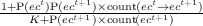
- P(ETTt) comes from the model described two sections above (7.5).
- P(ECt+1 = ec|ETTt = ett) =
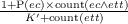
- P(Cct+1 = c|ECt+1 = ec) =
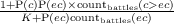 , we only count
when c won against ec.
, we only count
when c won against ec.
- Both P(Cft+1|TT) and P(λ|Cft+1,Cmt+1) are functions and do not need
identification.
Questions
The question that we ask to know which units to produce is:
or we can sample Ut+1 from P(Cft+1) or even from cft+1 (a realization of Cft=1) if
we ask P(Cft+1|eu1:Mt,ttt,λ = 1). Note that here we do not know fully neither the
value of ETT nor of Ct so we take the most information that we have into
account (distributions). The evaluation of the question is proportional to
 ×
× 2 ×|C|4 = V ′×K′2 ×K4. But we do not have to sum on the 4 types
of C in practice: P(Cm|Ct,Cc) is a simple linear combination of vectors and
P(λ = 1|Cf,Cm) is a linear filter function, so we just have to sum on Cc and
practical complexity is proportional to V ′× K′2 × K. As we have most often
≈ 10 Gaussian components in our GMM, K or K′ are in the order of 10
(5 to 12 in practice), while V and V ′ are between 211 and 517 as noted
above.
2 ×|C|4 = V ′×K′2 ×K4. But we do not have to sum on the 4 types
of C in practice: P(Cm|Ct,Cc) is a simple linear combination of vectors and
P(λ = 1|Cf,Cm) is a linear filter function, so we just have to sum on Cc and
practical complexity is proportional to V ′× K′2 × K. As we have most often
≈ 10 Gaussian components in our GMM, K or K′ are in the order of 10
(5 to 12 in practice), while V and V ′ are between 211 and 517 as noted
above.
Bayesian program
7.7.2 Results
We did not evaluate directly P(Ut+1|eut,ttt,λ = 1) the efficiency of the army
compositions which would be produced. Indeed, it is difficult to make it
independent from (at least) the specific micro-management of different unit types
composing the army. The quality of P(ETT) also has to be taken into account.
Instead, we evaluated the reduction of armies compositions (EU and U sets of
variables) into clusters (EC and C variables) and the subsequent P(Cc|EC)
table.
We use the dataset presented in section 6.4 in last chapter (tactics). It contains
everything we need about the state and battles, units involved, units lost, winners.
There are 7708 games. We only consider battles with about even force sizes, but that
lets a sizable number on the more than 178,000 battles of the dataset. For
each match-up, we set aside 100 test matches, and use the remaining of the
dataset for learning. We preferred robustness to precision and thus we did not
remove outliers: better scores can easily be achieved by considering only
stereotypical armies/battles. Performance wise, for the biggest dataset (PvT)
the learning part takes around 100 second on a 2.8 Ghz Core 2 Duo CPU
(and it is easily serializable) for 2408 games (57 seconds to fit and select the
GMM, and 42 seconds to fill the probability tables / fit the Categorical
distributions). The time to parse all the dataset is far larger (617 seconds with an
SSD).
Evaluation of clustering
We will look at the predictive power of the P(Cc|EC) (comprehending the reduction
from U to C and EU to EC) for the results of battles. For each battle, we
know the units involved (types and numbers) and we look at predicting the
winner.
Metrics
Each battle consists in numbers of units involved for each types and each parties (the
two players). For each battle we reduce the two armies to two Gaussian mixtures
(P(C) and P(EC)). To benchmark our clustering method, we then used the learned
P(Cc|EC) to estimate the outcome of the battle. For that, we used battles with
limited disparities (the maximum strength ratio of one army over the other) of
1.1 to 1.5. Note that the army which has the superior forces numbers has
more than a linear advantage over their opponent (because of focus
firing ),
so a disparity of 1.5 is very high. For information, there is an average of 5 battles per
game at a 1.3 disparity threshold, and the numbers of battles per game increase with
the disparity threshold.
We also made up a baseline heuristic, which uses the sum of the values of the
units (see section 6.3.2 for a reminder) to decide which side should win. If we note
v(unit) the value of a unit, the heuristic computes ∑
unitv(unit) for each army and
predicts that the winner is the one with the biggest score. Of course, we recall that a
random predictor would predict the result of the battle correctly 50% of the
time.
A summary of the main metrics is shown in Table 7.8, the first line can be
read as: for a forces disparity of 1.1, for Protoss vs Protoss (first column),
- considering only military units
- the heuristic predicts the outcome of the battle correctly 63% of the
time.
- the probability of a clusters mixture to win against another
(P(C|EC)), without taking the forces sizes into account, predicts the
outcome correctly 54% of the time.
- the probability of a clusters mixture to win against another, taking
also the forces sizes into account (P(C|EC)×∑
unitv(unit)), predicts
the outcome correctly 61% of the time.
- considering only all units involved in the battle (military units, plus static
defenses and workers): same as above.
And then it is given for all match-ups* (columns) and different forces disparities
(lines). The last column sums up the means on all match-ups, with the whole
army (military units plus static defenses and workers involved), for the three
metrics.
Also, without explicitly labeling clusters, one can apply thresholding to special
units (observers, arbiters, science vessels...) to generate more specific clusters: we did
not include these results here (they include too much expertize/tuning) but they
sometimes drastically increase prediction scores.
Predictive power
We can see that predicting battle outcomes (even with a high disparity) with “just
probabilities” of P(Cc|EC) (without taking the forces into account) gives relevant
results as they are always above random predictions. Note that this is a very high
level (abstract) view of a battle, we do not consider tactical positions, nor players’
attention, actions, etc. Also, it is better (in average) to consider the heuristic with
the composition of the army (prob×heuristic) than to consider the heuristic alone,
even for high forces disparity. These prediction results with “just prob.”, or
the fact that heuristic with P(Cc|EC) tops the heuristic alone, are a proof
that the assimilation of armies compositions as Gaussian mixtures of cluster
works.
Army efficiency
Secondly, and perhaps more importantly, we can view the difference between “just
prob.” results and random guessing (50%) as the military efficiency improvement
that we can (at least) expect from having the right army composition. Indeed, we see
that for small forces disparities (up to 1.1 for instance), the prediction with army
composition only (“just prob.”: 63.2%) is better that the prediction with the baseline
heuristic (61.7%). It means that we can expect to win 63.2% of the time
(instead of 50%) with an (almost) equal investment if we have the right
composition. Also, we predict 58.5% of the time the accurate result of a battle with
disparity up to 1.5 from “just prob.”: these predictions are independent of the
sizes of the armies. What we predicted is that the player with the better
army composition won (not necessarily the one with more or more expensive
units).
|
|
|
|
|
|
|
|
|
|
|
|
|
|
|
| forces | scores | PvP | PvT | PvZ | TvT | TvZ | ZvZ | mean |
| disparity | in % | m | ws | m | ws | m | ws | m | ws | m | ws | m | ws | ws |
|
|
|
|
|
|
|
|
|
|
|
|
|
|
|
| | heuristic | 63 | 63 | 58 | 58 | 58 | 58 | 65 | 65 | 70 | 70 | 56 | 56 | 61.7 |
| 1.1 | just prob. | 54 | 58 | 68 | 72 | 60 | 61 | 55 | 56 | 69 | 69 | 62 | 63 | 63.2 |
| | prob×heuristic | 61 | 63 | 69 | 72 | 59 | 61 | 62 | 64 | 70 | 73 | 66 | 69 | 67.0 |
|
|
|
|
|
|
|
|
|
|
|
|
|
|
|
| | heuristic | 73 | 73 | 66 | 66 | 69 | 69 | 75 | 72 | 72 | 72 | 70 | 70 | 70.3 |
| 1.3 | just prob. | 56 | 57 | 65 | 66 | 54 | 55 | 56 | 57 | 62 | 61 | 63 | 61 | 59.5 |
| | prob×heuristic | 72 | 73 | 70 | 70 | 66 | 66 | 71 | 72 | 72 | 70 | 75 | 75 | 71.0 |
|
|
|
|
|
|
|
|
|
|
|
|
|
|
|
| | heuristic | 75 | 75 | 73 | 73 | 75 | 75 | 78 | 80 | 76 | 76 | 75 | 75 | 75.7 |
| 1.5 | just prob. | 52 | 55 | 61 | 61 | 54 | 54 | 55 | 56 | 61 | 63 | 56 | 60 | 58.2 |
| | prob×heuristic | 75 | 76 | 74 | 75 | 72 | 72 | 78 | 78 | 73 | 76 | 77 | 80 | 76.2 |
|
|
|
|
|
|
|
|
|
|
|
|
|
|
|
| |
Table 7.8: Winner prediction scores (in %) for 3 main metrics. For
the left columns (“m”), we considered only military units. For the right
columns (“ws”) we also considered static defense and workers. The “heuristic”
metric is a baseline heuristic for battle winner prediction for comparison
using army values, while “just prob.” only considers P(Cc|EC) to predict
the winner, and “prob×heuristic” balances the heuristic’s predictions with
∑
Cc,ECP(Cc|EC)P(EC).
Analysis of the clustering
Figure 7.15 shows a 2D Isomap [Tenenbaum et al., 2000] projection of the
battles on a small ZvP dataset. Isomap finds a low-dimensional non-linear embedding
of the high dimensionality (N or N′ dimensions, as much as unit types, the length of
U or EU) space in which we represent armies. The fact that the embedding is
quasi-isometric allows us to compare the intra- and inter- clusters similarities. Most
clusters seem to make sense as strong, discriminating components. The clusters
identified by the numbers 2 and 7 (in this projection) are not so discriminative,
so they probably correspond to a classic backbone that we find in several
mixtures.
Figure 7.16 shows a parallel plot of army compositions. We removed the less frequent
unit types to keep only the 8 most important unit types of the PvP match-up, and
we display a 8 dimensional representation of the army composition, each vertical
axis represents one dimension. Each line (trajectory in this 8 dimensional
space) represents an army composition (engaged in a battle) and gives the
percentage
of each of the unit types. These lines (armies) are colored with their most probable
mixture component, which are shown in the rightmost axis. We have 8 clusters
(Gaussian mixtures components): this is not related to the 8 unit types used as the
number of mixtures was chosen by BIC* score. Expert StarCraft players
will directly recognize the clusters of typical armies, here are some of them:
- Light blue corresponds to the “Reaver Drop” tactical squads, which aims
are to transport (with the flying Shuttle) the slow Reaver (zone damage
artillery) inside the opponent’s base to cause massive economical damages.
- Red corresponds to the “Nony” typical army that is played in PvP (lots
of Dragoons, supported by Reaver and Shuttle).
- Green corresponds to a High Templar and Archon-heavy army: the gas
invested in such high tech units makes it that there are less Dragoons,
completed by more Zealots (which cost no gas).
- Purple corresponds to Dark Templar (“sneaky”, as Dark Templars are
invisible) special tactics (and opening).
Analysis of dynamics
Figure 7.17 showcases the dynamics of clusters components: P(ECt|ECt+1, for Zerg
(vs Protoss) for Δt of 2 minutes. The diagonal components correspond to those which
do not change between t and t + 1 (⇔ t + 2minutes), and so it is normal that they are
very high. The other components show the shift between clusters. For instance, the
first line seventh column (in (0,6)) square shows a brutal transition from
the first component (0) to the seventh (6). This may be the production of
Mutalisks
from a previously very low-tech army (Zerglings).
Extensions
Here, we focused on asking P(Ut+1|eut,ttt,λ = 1), and evaluated (in the absence of
ground truth for full armies compositions) the two key components that are P(U|C)
(or P(EU|EC)) and P(Cc|EC). Many other questions can be asked: P(TTt|eut)
can help us adapt our tech tree development to the opponent’s army. If we
know the opponent’s army composition only partially, we can benefit of
knowledge about ETT to know what is possible, but also probable, by asking
P(ECt|Observations).
7.8 Conclusion
We contributed a probabilistic model to be able to compute the distribution over
openings (strategies) of the opponent in a RTS game from partial and noisy
observations. The bot can adapt to the opponent’s strategy as it predicts the opening
with 63 - 68% of recognition rate at 5 minutes and > 70% of recognition rate at 10
minutes (up to 94%), while having strong robustness to noise (> 50% recognition rate
with 50% missing observations). It can be used in production due to its low CPU
(and memory) footprint.
We also contributed a semi-supervised method to label RTS game logs (replays) with
openings (strategies). Both our implementations are free software and can be found
online .
We use this model in our StarCraft AI competition entry bot as it enables it to deal
with the incomplete knowledge gathered from scouting.
We presented a probabilistic model inferring the best army composition given
what was previously seen (from replays, or previous games), integrating adaptation
to the opponent with other constraints (tactics). One of the main advantages of this
approach is to be able to deal natively with incomplete information, due to player’s
intentions, and to the fog of war in RTS. The army composition dimensionality
reduction (clustering) can be applied to any game and coupled with other techniques,
for instance for situation assessment in case-based planning. The results in battle
outcome prediction (from few information) shows its situation assessment
potential.
Chapter 8
BroodwarBotQ
Dealing with failure is easy: Work hard to improve. Success is also
easy to handled: You’ve solved the wrong problem. Work hard to
improve.
|
IN this chapter, we present some of the engineering that went in the
robotic player (bot) implementation, which may help the comprehension of the
organization and utility of the different chapters. We will also present the
different flows of informations and how decisions are made during a game.
Finally we will present the results of the full robotic player to various bots
competitions.
8.1 Code architecture
Our implementation (BSD
licensed) uses BWAPI
to get information from and to control StarCraft. The bot’s last major revision
(January 2011) consists of 23,234 lines of C++ code, making good use of boost
libraries and BWTA (Brood War Terrain Analyzer). The learning of the parameters
from the replays is done by separated programs, which serialize the probability
tables and distribution parameters, later loaded by BROODWARBOTQ each
game.
The global (simplified) view of the whole bot’s architecture is shown in
Figure 8.1. There are three main divisions: “Macro” (economical and production
parts), “Intelligence” (everything information related) and “Micro” (military units
control/actions). Units (workers, buildings, military units) control is granted through
a centralized Arbitrator to “Macro” parts and Goals. This is a bidding system in
which parts wanting a unit bid on it relatively to the importance of the
task they will assign it. There may (should) be better systems but it works.
We will now detail the parts which were explained in the previous three
chapters.
8.1.1 Units control
As presented in chapter 5, units are controlled in a sensory-motor fashion through
Bayesian fusion of physical or abstract influences. Units pursuing a common objective
are regrouped in a UnitsGroup, which sets this objective for every unit it commands.
This objective is generated for each unit from the needs of a higher-up Goal (see
below) through achieve() or cancel().
The BayesianUnit class has different fusion modes (see section 5.3.3) set by the
UnitsGroup depending on the Goal type and on the situation (number and types of
enemies, terrain...). Its sensory inputs are fed by the UnitsGroup (objectives) and by
the MapManager (potential damages, terrain) and the EUnitsFilter (enemy
units).
A derivative (child) of the BayesianUnit class is instantiated for each unit that is
controlled. A BayesianUnit is a modal FSM* as shown in Figure 5.7. It
presents a simple interface to move and fight (the micro() method). Some
parameter can be specialized depending on the particularities of unit types:
- the list of priority unit types to target (because of units attacks efficiencies
as in rock/paper/scissors),
- the reasons for which to flee (flee?()),
- micro() itself can be specialized further if the two points above do not
suffice to produce a skillful behavior (for very special unit types: casters).
A call to micro() then decides of the course of actions during a fight (applying Bayesian
fusion with the right sensory inputs when moving).
8.1.2 Tactical goals
The decision that we want our AI system to make at this level is where and how to
attack. This is reflected in the StarCraft bot as a Goal creation. Goals are interfacing
high level tactical thinking with the steps necessary to their realization. A Goal
recruits units and binds them under a UnitsGroup (see section 5.3.3). A Goal is an
FSM* in which two states are simple planners (an FSM with some form of procedural
autonomy), it has:
- preconditions, for instance a drop attack needs to specify at least a
transport unit (Shuttle/Dropship/Overlord) and ground attack units.
- hard states: waiting precondition, in progress, in cancel, achieved, canceled,
which corresponds to the Goal advancement..
- and and/or or logic subgoals with:
- a realization test
- a proposition of action to try to realize it
- an estimation of the “distance” to realization
In the in progress and in cancel modes, the “plan” is a simple search in the achievable
subgoals and their “distance” to realization.
The tactical model can specify where to attack by setting a localized subgoal
(Formation/See/Regroup/KillSubgoal...) to the right place. It can specify how by
setting the adequate precondition(s). It also specifies the priority of a Goal so that it
has can bid on the control of units relatively to its importance. The GoalManager
updates all Goals that were inputed and act as a proxy to the Arbitrator for
them.
8.1.3 Map and movements
The MapManager keeps track of:
- the economical and military bases (positions) of the enemy,
- the potential damages map, which is updated with each new observations
(units, spells...),
- the “walkability” of the terrain (static terrain and buildings).
It also provides threaded pathfinder services which are used by UnitsGroups to generate
objectives waypoints when the Goal’s objectives are far. This pathfinder can be asked
specifically to avoid certain zones or tiles.
8.1.4 Technology estimation
The ETechEstimator does constant build tree* prediction as explained in
section 7.5, and so it exposes the distribution on the enemy’s tech tree* as a “state
estimation service” to other parts of the bot taking building and production decision.
It also performs openings* prediction during the first 15 minutes of the game, as
explained in section 7.6.
New enemy units observations are taken into account instantly. When we see an
enemy unit at time t, we infer that all the prerequisites were built at least
some time t′ earlier according to the formula: t′ = t - ubd - umd with ubd
being the unit’s building duration (depending on the unit type), and umd
being the unit’s movement duration depending on the speed of the unit’s
type, and the length of the path from its current position to the enemy’s
base. We can also observe the upgrades that the units have when we see
them, and so we take that into account the same way. For instance, if a unit
has an attack upgrade, it means that the player has the require building
since at least the time of observation minus the duration of the upgrade
research.
The distribution on openings* computed by the ETechEstimator serves the
purpose of recognizing the short term intent of the enemy. This way, the
ETechEstimator can suggest the production of counter measures to the opponent’s
strategy and special tactics. For instance, when the belief that the enemy is doing a
“Dark Templars” opening (an opening aimed at rushing invisible technology before
the time at which a standard opening reaches detector technology, to inflict massive
damage) pass above a threshold, the ETechEstimator suggests the construction of
turrets (Photon Cannon, static defense detectors) and Observers (mobile
detectors).
8.1.5 Enemy units filtering
At the moment, enemy units filtering is very simple and just diffuse uniformly (with
respect to its speed) the probability of a unit to be where it was last seen before
totally forgetting about its position (not its existence) when it was not seen for
too long. We will now shortly present an improvement to this enemy units
tracking.
A possible improved enemy units tracking/filtering
We consider a simple model, without speed nor steering nor See variable for each
position/unit. The fact that we see positions where the enemy units are is taken into
account during the update. The idea is to have (learn) a multiple influences
transition matrix on a Markov chain on top of the regions discretization (see
chapter 6), which can be seen as one Markov chain for each combination of
motion-influencing factors.
The perception of such a model would be for each unit if it is in a given
region, as the bottom diagram in Figure B.2. From there, we can consider
either map-dependent regions, regions uniquely identified as they are in
given maps that is; or we can consider regions labeled by their utility. We
prefer (and will explain) this second approach as it allows our model to be
applied on unknown (never seen) maps directly and allows us to incorporate
more training data. The regions get a number in the order in which they
appear after the main base of the player (e.g. see region numbering in Fig. 6.2
and 8.2).
Variables
The full filter works on n units, each of the units having a mass in the each of the m
regions.
- Agg ∈ {true,false}, the player’s aggressiveness (are they attacking or
defending?), which can comes from other models but can also be an output
here.
- UTi∈⟦1…n⟧ ∈{unit types} the type of the ith tracked unit, with K unit
types.
- Xi∈⟦1…n⟧t-1 ∈⟦r1…rm⟧, the region in which is the ith unit at time t - 1.
- Xi∈⟦1…n⟧t ∈⟦r1…rm⟧, the region in which is the ith unit at time t.
Joint Distribution
We consider all units conditionally independent give learned parameters. (This may
be too strong an assumption.)
Forms
- P(Agg) = Binomial(pagg) is a binomial distribution.
- P(UTi) = Categorical(K,put) is categorical distribution (on unit types).
- P(Xit-1) = Categorical(m,preg) is a categorical distribution (on regions).
- P(Xit|Xit-1,UTi,Agg) are #{units_types}×
 = K × 2 different
m×m matrices of transitions from regions to other regions depending on
the type of unit i and of the aggressiveness of the player. (We just have
around 15 unit types per race (K ≈ 15) so we have ≈ 15 × 2 different
matrices for each race.)
= K × 2 different
m×m matrices of transitions from regions to other regions depending on
the type of unit i and of the aggressiveness of the player. (We just have
around 15 unit types per race (K ≈ 15) so we have ≈ 15 × 2 different
matrices for each race.)
Identification (learning)
P(Xit|Xit-1,UTi,Agg) is learned with a Laplace rule of succession from
previous games. Against a given player and/or on a given map, one can use
P(Xit|Xit-1,UTi,Agg,Player,Map) and use the learned transitions matrices as
priors. When a player attacks in the dataset, we can infer she was aggressive at the
beginning of the movements of the army which attacked. When a player gets
attacked, we can infer she was defensive at the beginning of the movements of the
army which defended. At other times, P(Agg = true) = P(Agg = false) = 0.5.
Note that we can also (try to) learn specific parameters of this model during
games (not a replay, so without full information) against a given opponent with
EM* to reconstruct and learn from the most likely state given all the partial
observations.
Update (filtering)
- When a unit i becomes hidden, which was seen in region r just before, we have:
- For all regions r that we see “totally” (above a threshold of a percentage of the
total area), we set P(Xit = r) = 0.0 and redistribute their probability mass to
hidden (or still partially hidden) regions (algorithm 6):
Algorithm 6: Culling/updating algorithm for filtering visible regions
for all i ∈{enemy_units} do s ← 0.0 for all r ∈{visible_regions} do s ← s + P(Xit-1 = r) P(Xit-1 = r) = 0.0 end for total ←∑ j=1mP(Xit-1 = rj) for all r ∈{¬visible_regions} do P(Xit = r) ← P(Xit = r) +  × P(Xit-1 = r) end for end for
- For all the other cases, we have:
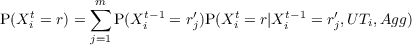
Questions
- When we want to infer where the n enemy units are, we ask:
- When we want to infer the aggressiveness of the enemy (from the troupes’
movements that we have seen), we ask:
Conclusion
Offline learning of matrices (as shown in Fig. 8.2) of aggressive and defensive
probable region transitions (for a given unit type). With online learning (taking
previous offline learned parameters as priors), we could learn preferences of a given
opponent.
By considering a particle filter [Thrun, 2002], we could consider a finer model in
which we deal with positions of units (in pixels or walk tiles or build tiles) directly,
but there are some drawbacks:
- The data to learn (offline or online) is sparse as there are several versions
of the same map and the combinatorics of start positions (2 occupied start
positions on 4 possible most of the time). This would need any form of
spatial abstraction anyway, like distance to most walked traces.
- Computation cost to track ≈ 40 units makes it so that the particle
sampling numbers should be low to stay real-time. Or that one should
abandon the motion model for a Kalman filter [Kalman, 1960].
The advantages are not so strong:
- (hopefully) more precision in units position estimation,
- possibilities to have more complex motion models (updates/culling of the
filter),
- differentiation between trajectories of ground and flying units,
- differentiation between different trajectories of attacks inside large regions.
We would like to implement our regions-based enemy units filtering in the future, mainly
for more accurate and earlier tactical prediction (perhaps even drop tactics
interception) and better tactical decision making.
8.2 A game walk-through
We will now show key moments of the game, as was done with a human-played game
in section 4.1.2, but from the bot’s point of view (with debug output).
First, Figure 8.3 shows some economical elements of BBQ. The yellow rectangles
show future buildings placements. In the light blue (teal color) rectangle are the next
buildings which are planned for construction with their future positions. Here, the
Protoss Pylon was just added to the construction plan as our Producer estimated
that we will be supply* blocked in 28 seconds at the current production rate. This is
noted by the “we need another pylon: prevision supply 84 in 28 sec” line, as
supply is shown doubled (for programmatic reasons, so that supply is always
an integer): 84 is 42, and we have a current max supply* of 41 (top right
corner).
Our buildings placer make it sure that there is always a path around our
buildings blocks with a flow algorithm presented in the appendix in algorithm 9 and
Figure B.7. It is particularly important to be able to circulated in the base, and that
newly produced units are not stuck when they are produced (as they could is there
was a convex enclosure as in Fig. B.7). Buildings cannot be placed anywhere on the
map, even more so for Protoss buildings, as most of them need to be build under
Pylon coverage (the plain blue ellipses in the screenshot). At the same time,
there are some (hard) tactical requirements for the placement of defensive
buildings .
At the beginning of the game, we have no idea about what the opponent is doing
and thus our belief about their opening equals the prior (here, we set the priori to be
uniform, see section 7.6.3 for how we could set it otherwise) we send a worker unit to
“scout” the enemy’s base both to know where it is and what the enemy is up to.
Figure 8.4 shows when we first arrive at the opponent’s base in a case in which we
have a strong evidence of what the opponent is doing and so our beliefs are heavily
favoring the “Fast Legs” opening (in the blue rectangle on the right). We can see
that with more information (the bottom picture) we make an even stronger
prediction.
If our bot does not have to defend an early rush by the opponent, it chooses to do
a “push” (a powerful attack towards the front of the opponent’s base) once it
has a sufficient amount of military units, while it expands* (take a second
base) or opens up its tech tree*. The first push is depicted in Figure 8.5:
- First (top), we regroup our forces in front of the opponent’s base with a
formation SubGoal.
- By trying to enter the opponent’s base (second screenshot), our units have
to fight they way through.
- The bottom left picture shows the distribution on P(Diri) for the possible
movements directions of one of the units at the top. We can see that it
wants to avoid collision with allied units while going towards its target.
- The bottom right picture shows our units “kiting back” (retreating while
fighting) to avoid being exposed in the ramp up the cliff (right part of the
image).
BroodwarBotQ then goes up the ramp and destroys the base of the built-in
AI.
8.3 Results
BroodwarBotQ (BBQ) consistently beats the built-in StarCraft: Broodwar
AI ,
to a point that the original built-in AI is only used to test the stability of our bot,
but not as a sparing/training partner.
BroodwarBotQ took part in the Artificial Intelligence and Interactive Digital
Entertainment (AAAI AIIDE) 2011 StarCraft AI competition. It got 67 games
counted as “crashes” on 360 games because of a misinterpretation of rules on the first
frame ,
which is not the real unstability of the bot (≈ 0,75% as seen in B.8). The results of
AIIDE are in Table 8.1.
|
|
|
|
|
| bot | race | refs | win rate | notes |
|
|
|
|
|
| Skynet | Protoss | | 0.889 | openings depending on opponent’s race |
| UAlbertaBot | Protoss | [Churchill and Buro, 2011] | 0.794 | always 2-Gates opening |
| Aiur | Protoss | | 0.703 | robust and stochastic strategies |
| ItayUndermind | Zerg | | 0.658 | 6-pooling |
| EISBot | Protoss | [Weber et al., 2010b,a] | 0.606 | 2-Gates or Dragoons opening |
| SPAR | Protoss | [Kabanza et al., 2010] | 0.539 | uses Dark Templars |
| Undermind | Terran | | 0.517 | Barracks units |
| Nova | Terran | [Pérez and Villar, 2011] | 0.475 | robust play |
| BroodwarBotQ | Protoss | | 0.328 | adapts to the opening |
| BTHAI | Zerg | [Hagelbäck and Johansson, 2009] | 0.319 | Lurkers opening |
| Cromulent | Terran | | 0.300 | Factory units |
| bigbrother | Zerg | | 0.278 | Hydralisks and Lurkers |
| Quorum | Terran | | 0.094 | expands and produce Factory units |
|
|
|
|
|
| |
Table 8.1: Result table for the AIIDE 2011 StarCraft AI competition with 360
games played by each bot.
Also in 2011 was the Computational Intelligence and Games
(IEEE CIG) 2011 StarCraft AI competition. This competition had 10
entries
and BroodwarBotQ placed 4th with a little luck of seed (it did not have to play
against Aiur). The finals are depicted in Table 8.2.
|
|
|
|
|
| bot | race | crashes | games | wins |
|
|
|
|
|
| Skynet | Protoss | 0 | 30 | 26 |
| UAlbertaBot | Protoss | 0 | 30 | 22 |
| Xelnaga | Protoss | 3 | 30 | 11 |
| BroodwarBotQ | Protoss | 2 | 30 | 1 |
|
|
|
|
|
| |
Table 8.2: Result table of the finals for the CIG 2011 StarCraft AI competition
(10 entries)
Finally, there is a continuous ladder in which BroodwarBotQ (last updated
January 2012) is ranked between 7 and 9 (without counting duplicates, there are ≈
20 different bots) and is on-par with EISBot [Weber et al., 2010b,a] as can be
seen in Figure B.8 (February 2012 ladder ranking). We consider that this
rating is honorable, particularly considering our approach and the amount
of engineering that went in the other bots. Note that the ladder and all
previous competitions do not allow to record anything (learn) about the
opponents.
We want to give a quick analysis of the performance of BroodwatBotQ. We did
not specialize the bot for one (and only one) strategy and type of tactics, which
makes our tactics less optimized than other concurrents higher up in the
ladder. Also, our bot tries to adapts its strategy, which has two drawbacks:
- our strategy prediction model’s parameters were learned from
human-played games, which differ from bot’s games.
- some of the decision-making (particularly with regard to arbitrage of
resources) is not probabilistic and interfaces badly with the predictions
and suggestions. For instance, when we predict a “Dark Templars” opening,
the ETechEstimator suggests building static and mobile detectors, both
may be out of our current tech tree*: how do we allocate our (limited)
resources and plan the constructions, while taking into consideration the
current building and production plan? This is not solved currently in a
unified manner.
Chapter 9
Conclusion
Man’s last mind paused before fusion, looking over a space that
included nothing but the dregs of one last dark star and nothing besides
but incredibly thin matter, agitated randomly by the tag ends of heat
wearing out, asymptotically, to the absolute zero.
Man said, “AC, is this the end? Can this chaos not be reversed into the
Universe once more? Can that not be done?”
AC said, “THERE IS AS YET INSUFFICIENT DATA FOR A
MEANINGFUL ANSWER.”
Isaac Asimov (The Last Question, 1956)
|
9.1 Contributions summary
We classified the problems raised by game AI, and in particular by RTS AI. We
showed how the complexity of video games makes it so that game AI systems can
only be incompletely specified. This leads to uncertainty about our model, but also
about the model of the opponent. Additionally, video games are often partially
observable, sometimes stochastic, and most of them require motor skills (quick and
precise hands control), which will introduce randomness in the outcomes of player’s
actions. We chose to deal with incompleteness by transforming it into uncertainty
about our reasoning model. We bind all these sources of uncertainty in Bayesian
models.
Our contributions about breaking the complexity of specifying and controlling
game AI systems are resumed by:
- In chapter 5, we produced reactive, decentralized, multi-agent control
by transforming the incompleteness about allied units intentions into
uncertainty of their future locations. This can be viewed as an
extension of Bayesian robot programming [Lebeltel et al., 2004] in
a multi-agent setting. Instead of specifying a distribution on the
possible directions knowing the sensory inputs, we specified the sensor
distribution (independently of each other sensors) knowing the direction
(P(Sensor|Direction)). This approach, called inverse programming, can
be viewed as “instead of specifying the states and their transitions
based on sensors (an FSM), we specifying what the sensors should
be when we are in a given state”, reverting some of the burden of
specifying behaviors, and in a probabilistic setting. This is an extension
of the work on inverse programming for Unreal Tournament avatars
[Le Hy et al., 2004]. Combined, these contributions lead to real-time
micro-management behaviors for StarCraft, which achieved very satisfying
results (ex-aequo with the best micro-management AI of AIIDE 2010
competition), and were published in [Synnaeve and Bessière, 2011a].
- By going up in the ladder of abstraction (strategy & tactics), we were able
to exploit what we previously called vertical continuity (see section 2.8.1)
through hierarchical models. About strategy (chapter 7), from low-level
observations, we produced build trees* (section 7.5, [Synnaeve and
Bessière, 2011]), and built upon that to infer openings* (section 7.6,
[Synnaeve and Bessière, 2011b]) and to constrain the inference on the
opponent’s army composition (section 7.7). Tactics (chapter 6) also make
good use of the prediction on the opponent’s tech tree*. When used in
decision-making, our models are even more constrained, because we have
full knowledge of our state instead of distributions.
- We also took advantage of actions sequencing, previously called horizontal
continuity (see section 2.8.1), by assessing that, often, things which are
done should not be undone (at least not immediately) and that some
strategic and tactical steps are prerequisite of intended steps. At the
strategic level, the distribution on build trees* is time-dependent: the
sequencing is encoded in the learned discrete Gaussian distributions
(section 7.5, [Synnaeve and Bessière, 2011]). The openings are filtered on
previous inferences with a first order Markovian assumption (section 7.6,
[Synnaeve and Bessière, 2011b]), i.e. the value at time t is dependent
on the value at time t - 1. The army composition model (section 7.7)
makes use of temporal continuity to adapt the player’s army to
the opponent’s future army composition. Micro-management assumes
an uncertain linear interpolation of future units position resulting of
trajectory continuity (instead of considering all possible positions), as
explained in subsection 5.3.1.
We used machine learning to help specifying our models, both used for prediction
(opponent modeling) and for decision-making. We exploited different datasets for
mainly two separate objectives:
- We produced relevant abstract models thanks to learning. For the
labeling replays (allowing for supervised learning of our full openings*
prediction model), we used semi-supervised (by selecting features and a
scoring function) GMM* clustering of replays, as presented in section 7.4
[Synnaeve and Bessière, 2011b]. In order to reason qualitatively and
quantitatively about armies composition with a tractable model, we
applied GMM to armies unit types percentages to find the different
composing components (section 7.7). For tactics, we used heuristics
(see subsection 6.3.2) for the evaluation of the regions, whose bias
(incompleteness) the model was adapted to by learning.
- We learned the parameters of our models from human-played games
datasets. At the strategic level, we learned the time-dependent
distributions on the build trees and the co-occurrence of openings with
build trees in sections 7.5 and 7.6, respectively published as [Synnaeve
and Bessière, 2011], [Synnaeve and Bessière, 2011b]. We were also able to
study the strengths and weaknesses of openings this way (subsection 7.6.2,
and we looked at the dynamics or army compositions (section 7.7). For
tactics (see chapter 6), we learned the co-occurrences of attacks with
regions tactical properties.
Finally, we produced a StarCraft bot (chapter 8), which ranked 9th (on 13) and
4th (on 10), respectively at the AIIDE 2011 and CIG 2011 competitions. It is about
8th (on ≈ 20) on an independent ladder containing all bots submitted to
competitions (see Fig. B.8).
9.2 Perspectives
We will now present interesting perspectives and future work by following our
hierarchical decomposition of the domain. Note that there are bridges between the
levels presented here. In particular, having multi-scale reasoning seems necessary to
produce the best strategies. For instance, no current AI is able to work out a “fast
expand*” (expand before any military production) strategy by itself, in which it
protects against early rushes by a smart positioning of buildings, and it performs
temporal reasoning about when the opponent is first a threat. This kind of reasoning
encompasses micro-management level reasoning (about the opponent units), with
tactical reasoning (of where and when), buildings positioning, and economical and
production planning.
9.2.1 Micro-management
Reactive behaviors
An improvement (explained in subsection 5.6.1) over our existing model usage
would consist in using the distributions on directions (P(Dir)) for each units
to make a centralized decision about which units should go where. This
would allow for coordinated movements while retaining the tractability of a
decentralized model: the cost for units to compute their distributions on directions
(P(Dir)) is the same as in the current model, and there are methods to select
the movements for each unit which are linear in the number of units (for
instance maximizing the probability for the group, i.e. for the sum of the
movements).
For the problem of avoiding local optima “trapping”, we proposed a “trailing
pheromones repulsion” approach in subsection 5.6.1 (see Fig. 5.14), but other
(adaptive) pathfinding approaches can be considered.
Parameters identifications
Furthermore, the identification of the probability distributions of the sensors knowing
the directions (P(Sensor|Direction)) is the main point of possible improvements. In
the industry, behavior could be authored by game designers equipped with an
appropriate interface (with “sliders”) to the model’s parameters. As a competitive
approach, reinforcement leaning or evolutionary learning of the probability tables (or
probability distributions’ parameters) seems the best choice. The two main problems
are:
- types and/or levels of opponents: as we cannot assume optimal play from
the opponents (at least not for large scale battles), the styles and types of
the opponents’ control will matter for the learning.
- differences in situations: as there are several types of micro-management
situations, we have to choose the granularity of learning settings (battles)
and how we recognize them in-game. We could consider the continuum of
situations, and use Bayesian fusion of posteriors from models learned in
discrete contexts.
As the domain (StarCraft) is large, distributions have to be efficiently parametrized
(normal, log-normal, exponential distributions should fit our problem). The two main
approaches to learn these sensors distributions would be:
- Concurrent hierarchical reinforcement learning ([Marthi et al., 2005]
showed how it can work in Wargus).
- Co-evolving control policies by playing them against each others ([Miles
et al., 2007, Avery et al., 2009] presented a related work with influence
maps).
.
9.2.2 Tactics
We explained the possible improvements around our model in subsection 6.7.2. The
three most interesting research directions for tactics would be:
- Improve tactical state estimation,
so that both our tactical decision-making and tactical prediction benefit
from it. A first step would be to use a (dynamic) filtering on enemy units.
We proposed a simpler units filtering model based on the decomposition
of the map in regions in section 8.1.5.
- Use our learned parameters as bootstrap (“prior”) and keep on learning
against a given opponent and/or on a given map. We should count how
often and in which circumstances an attack, which should be successful,
fails. It should even be done during a given game (as human players do).
This may be seen as an exploration-exploitation trade-off in which our
robotic player wants to minimize its regret for which multi-armed bandits
[Kuleshov and Precup, 2000] are a good fit.
- Tactical assault generation, so that we do not have to hard-code
the tactical goals behaviors. The definition of tactics used in [Ponsen
et al., 2006] is not exactly matching ours, but they evolved some strategic
and tactical decision elements (evolving knowledge bases for CBR*) in
Wargus. However, we are still far from script-independent tactics (in
StarCraft). Being able to infer the necessary steps to carry out a Drop
(request a Dropship and military units, put them in the Dropship at some
location A and drop them at location B to attack location C, retreat if
necessary) attack would be a good benchmark for tactics generation.
9.2.3 Strategy
Higher-level parameters as variables
Strategy is a vast subject and impacts tactics very much. There are several “strategic
dimensions”, but we can stick to the two strategy axes: aggressiveness (initiative),
and economy/technology/production balance. These dimensions are tightly coupled
inside a strategical plan, as putting all our resources in economy at time t is not
aimed at attacking at time t + 1. Likewise, putting all our resources in military
production at time t is a mistake if we do not intend to be aggressive at time t + 1.
However, there are several combinations of values along these dimensions, which lead
to different strategies. We detailed these higher order views of the strategy in
section 7.1.
In our models (tactics & army composition), the aggressiveness is a parameter.
Instead these two strategic dimensions could be encoded in variables:
- A ∈ {true,false} for the aggressiveness/initiative, which will influence
tactical (When do we attack?) and strategic models (How much do we
adapt and how much do we follow our initiative? How do we adapt?).
- ETP ∈{eco,tech,prod} which will arbitrate how we balance our resources
between economic expansion, technology advances and units production.
A possibility is yet again to try and use a multi-armed bandit acting on this two
variables (A and ETP), which (hyper-)parametrize all subsequent models. At this
level, there is a lot of context to be taken into account, and so we should specifically
consider contextual bandits.
Another interesting perspective would be to use a hierarchy (from strategy to
tactics) of reinforcement learning of (all) the bot’s parameters, which can be seen as
learning the degrees of liberty (of the whole bot) one by one as in [Baranès and
Oudeyer, 2009]. A more realistic task is to learn only these parameters that we
cannot easily learn from datasets or correspond to abstract strategical and tactical
thinking (like A and ETP).
Production & construction planning
A part of strategy that we did not study here is production planning, it encompasses
planning the use (and future collection) of resources, the construction of buildings
and the production of units. Our bot uses a simple search, some other bots
have more optimized build-order search, for instance UAlbertaBot uses a
build-order abstraction with depth-first branch and bound [Churchill and
Buro, 2011]. Planning can be considered (and have been, for instance [Bartheye and
Jacopin, 2009]), but it needs to be efficient enough to re-plan often. Also, it
could be interesting to interface the plan with the uncertainty about the
opponent’s state (Will we be attacked in the next minute? What is the opponent’s
technology?).
A naive probabilistic planning approach would be to plan short sequences of
constructions as “bricks” of a full production plan, and assign them probability
variables which will depend on the beliefs on the opponent’s states, and
replan online depending on the bricks probabilities. For instance, if we are
in a state with a Protoss Cybernetics Core (and other lower technology
buildings), we may have a sequence “Protoss Robotics Facility → Protoss
Observatory” (which is not mutually exclusive to a sequence with Protoss Robotics
Facility only). This sequence unlocks detector technology (Observers are
detectors, produced out of the Robotics Facility), so its probability variable (RO)
should be conditioned on the belief that the opponent has invisible units
(P(RO = true|Opening = DarkTemplar) = high or parametrize P(RO|ETT)
adequately). The planner would both use resources planning, time of construction,
and this posterior probabilities on sequences.
9.2.4 Inter-game Adaptation (Meta-game)
In a given match, and/or against a given player, players tend to learn from their
immediate mistakes, and they adapt their strategies to each other’s. As
this can be seen as a continuous learning problem (reinforcement learning,
exploration-exploitation trade-off), there is more to it. Human players call this the
meta-game*, as they enter the “I think that he thinks that I think...” game
until arriving at fixed points. This “meta-game” is closely related to the
balance of the game, and the fact that there are several equilibriums makes the
interest of StarCraft. Also, clearly, for human players there is psychology
involved.
Continuous learning
For all strategic models, the possible improvements (subsections 7.5.3, 7.6.3, 7.7.2)
would include to learn specific sets of parameters against the opponent’s strategies.
The problem here is that (contrary to battles/tactics) there are not much
observations (games against a given opponent) to learn from. For instance, a
naive approach would be to learn a Laplace’s law of succession directly on
P(ETechTrees = ett|Player = p) =  , and do the same for
EClusters, but this could require several games. Even if we see more than one tech
tree per game for the opponent, a few games will still only show a sparse subset of
ETT. Another part of this problem could arise if we want to learn really in-game as
we would only have partial observations.
, and do the same for
EClusters, but this could require several games. Even if we see more than one tech
tree per game for the opponent, a few games will still only show a sparse subset of
ETT. Another part of this problem could arise if we want to learn really in-game as
we would only have partial observations.
Manish Meta [2010] approached “meta-level behavior adaptation in RTS games”
as a mean for their case-based planning AI to learn from its own failures in Wargus.
The opponent is not considered at all, but this could be an interesting entry point to
discover bugs or flaws in the bot’s parameters.
Bot’s psychological warfare
Our main idea for real meta-game playing by our AI would be to use our models
recursively. As for some of our models (tactics & strategy), that can be used both for
prediction and decision-making, we could have a full model of the enemy by
maintaining the state of a model from them, with their inputs (and continually learn
some of the parameters). For instance, if we have our army adaptation model for
ourselves and for the opponent, we need to incorporate the output of their model as
an input of our model, in the part which predicts the opponent’s future
army composition. If we cycle (iterate) the reasoning (“I will produce this
army because they will have this one”...), we should reach these meta-game
equilibriums.
Final words
Finally, bots are as far from having a psychological model of their opponent as from
beating the best human players. I believe that this is our adaptability, our continuous
learning, which allows human players (even simply “good” ones like me) to beat RTS
games bots consistently. When robotic AI will start winning against human players,
we may want to hinder them to have only partial vision of the world (as humans do
through a screen) and a limited number of concurrent actions (humans use a
keyboard and a mouse so they have limited APM*). At this point, they will need an
attention model and some form of hierarchical action selection. Before that, all the
problems arose in this thesis should be solved, at least at the scale of the RTS
domain.
Glossary
-
AI directors
- system that overlooks the behavior of the players to manage the
intensity, difficulty and fun. 22
-
APM
- action per minute, an input speed frequency in competitive gaming. 78,
239, 242, 436
-
Bayesian game
- a game in which information about knowledge about payoffs
is incomplete. 58, 66
-
BIC
- Bayesian information criterion, a score for model selection. For a given
model with n data points, k parameters and L the maximum likelihood,
BIC = -2ln(L) + k ln(n). 305, 307, 385
-
BP
- Bayesian program. 98
-
branching factor
- (average) number of nodes at each level of a search tree, i.e.
base b of the complexity of a search of depth d in a tree, which is O(bd).
13, 36, 43, 44, 66
-
build order
- a formal specification of timings (most often indexed on total
population count) at which to perform build actions in the early game..
133, 290, 296
-
build tree
- abbrev. for “buildings tree”, state of the buildings (and thus
production) unlocked by a player. 127, 285, 289–291, 320, 340, 354, 366,
367, 401, 430
-
BWAPI
- Brood War Application Programmable Interface. 239
-
BWTA
- BroodWar Terrain Analyser. 229, 459
-
CBR
- Case-Based Reasoning. 228, 289, 433
-
Dark Spore
- a fast-paced, sci-fi action-RPG, with PvP and cooperative (vs AI)
modes. 22
-
DSL
- Domain Specific Language. 23
-
EM
- expectation-maximization, an iterative method to optimize parameters of
statistical models depending on unobserved variables. The expectation
(E) step gives the likelihood depending on the latent variables, and
the maximization (M) step computes maximizing parameters for the
expectation of this likelihood.. 298, 305, 306, 404
-
expand
- either placement of a new base or the action to take a new base (to
collect more resources).. 147, 419, 431
-
fog of war
- hiding of some of the features (most often units and new buildings)
for places where a player does not have units in range of sight.. 22, 64, 77,
128, 129, 147, 232, 469
-
FPS
- First Person Shooter: egocentric shooter game, strong sub-genres are fast
FPS, also called “Quake-likes”, e.g. Quake III; and team/tactical FPS, e.g.
Counter-Strike, Team Fortress 2. 21, 63, 77, 78, 82, 89, 215
-
FSM
- finite state machine. 23, 60, 176, 289, 399
-
gameplay
- describes the interactive aspects of game design, which constraints
the players possible behaviors and the players’ goals in a given game. Also,
the category/type of the game.. 20, 59, 127, 128, 215
-
gamification
- the use of game mechanics and game design to enhance non-game
contexts. 22
-
gas
- also called vespene, short for vespene gas. Advanced resource in StarCraft,
use for all advanced units, technological buildings, upgrades and
researches. It can be harvested only once an assimilator/refinery/extractor
has been built on the gas geyser and maximally fast with 3 workers only
at the closest (standard) distance to the resource depot.. 127, 130, 132,
243
-
GMM
- Gaussian mixture model, a generative model in which observations are
the outcomes of mixtures of normal distribution.. 298, 305, 430
-
goban
- board used for the game of Go. 44
-
HFSM
- hierarchical finite state machine. 23, 186
-
HMM
- Hidden Markov Model, a dynamic Bayesian network estimating hidden
states following a Markov process from observations. 90, 290
-
HTN
- hierarchical task network. 23, 61, 290
-
Left 4 Dead
- a teamplay (cooperative vs AI) survival horror FPS in which
players have to fight and escape zombie hordes. 22
-
match-up
- the pairing of two factions in StarCraft for a match in the form XvY,
with X and Y being factions. When we consider only one race’s strategy,
it should be in front. For instance, PvT is the Protoss versus Terran
match-up, with Protoss being studied if the features are not symmetric..
293, 304, 319, 331, 350, 363, 367, 378
-
max supply
- also total supply, maximum number of units that a player can
control at a given time, can be increased up to a hard limit (200 in
StarCraft).. 130, 132, 243, 413
-
MCMC
- Monte-Carlo Markov chain. 282
-
MCTS
- Monte-Carlo Tree Search. 44, 47, 282
-
MDP
- Markov decision process. 77
-
meta-game
- preparation and maneuvering before (and between) games
to exploit: current trends, opponent’s style and weaknesses, map’s
specificities (safe zones, back doors, timings), and psychological “mind
games”.. 435
-
micro-management
- gameplay actions that are manually addressed by the
player; the way of maximizing one’s army efficiency by using the units to
the maximum of their potential.. 127, 143, 147, 157, 160, 161, 165, 175,
485
-
mineral
- basic resource in StarCraft, used for everything. It can be harvested
increasingly faster with the number of workers (up to an asymptote).. 127,
130, 132, 243
-
mini-map
- radar view of the full game area, shown in the bottom corner of the
interface in StarCraft.. 132
-
MMORPG
- Massively Multi-player Online Role Playing Game, distinct of
RPG by the scale of cooperation sometimes needed to achieve a common
goal, e.g. Dark Age of Camelot, World of Warcraft. 21, 89, 100, 101
-
NPC
- non-playing characters: game AI controlled third party characters, which
were not conceived to be played by humans by opposition to “bots”. 20–22,
124
-
opening
- in Chess as in RTS games: the first strategic moves of the game, the
strategy of the early game. 133, 142, 144, 289, 291, 292, 298, 350, 401, 430
-
partisan
- (game) which is not impartial, in which a player can do actions
another can not do (move a faction while the other player(s) cannot). 36
-
perfect-information
- (game) in which all the players have complete knowledge
of the (board) state of the game. 36
-
POMDP
- partially observable Markov decision process. 77, 78, 157, 223
-
positional hashing
- a method for determining similarities in (board) positions
using hash functions. 53
-
pro-gamer
- professional gamer, full-time job. 21, 128
-
PvE
- Players vs Environment. 22, 62, 101
-
PvP
- Players versus Players. 22
-
replay
- the record of all players’ actions during a game, allowing the game
engine to recreate the game state deterministically. 21, 129, 239, 243, 292
-
replayability
- replay value, entertainment value of playing the game more than
once. 22
-
RL
- reinforcement learning. 166
-
RPG
- Role Playing Game, e.g. Dungeons & Dragons based Baldur’s Gate. 21,
63, 78, 82, 215
-
RTS
- Real-Time Strategy games are (mainly) allocentric economic and military
simulations from an operational tactical/strategist commander viewpoint,
e.g. Command & Conquer, Age of Empires, StarCraft, Total Annihilation.
13, 14, 21, 77, 78, 82
-
rush
- quick aggressive opening. 291
-
solved game
- a game whose outcome can be correctly predicted from any
position when each side plays optimally. 25
-
StarCraft: Brood War
- a science fiction real-time strategy (RTS) game
released in 1998 by Blizzard Entertainment. 21
-
supply
- cost in population (or supply) of a given unit, or current population
count of a player. Originally, the Terran name for population/psi/control..
130, 132, 243, 413
-
tech tree
- abbreviation for “technological tree”, state of the technology
(buildings, researches, upgrades) which are unlocked/available to a given
player.. 127, 130, 142, 147, 232, 235, 237, 275, 285, 288–291, 367, 368, 401,
419, 426, 430, 472
-
UCT
- Upper Confidence Bounds for Trees. 47, 282
-
zero-sum game
- a game in which the total score of each players, from one
player’s point-of-view, for every possible strategies, adds up to zero; i.e.
“a player benefits only at the expense of others”. 25
Bibliography
David W. Aha, Matthew Molineaux, and Marc J. V. Ponsen. Learning
to win: Case-based plan selection in a real-time strategy game. In Héctor
Muñoz-Avila and Francesco Ricci, editors, ICCBR, volume 3620 of Lecture
Notes in Computer Science, pages 5–20. Springer, 2005. ISBN 3-540-28174-6.
no citations
Srinivas M. Aji and Robert J. McEliece. The generalized distributive law.
IEEE Transactions on Information Theory, 46(2):325–343, 2000. no citations
David W. Albrecht, Ingrid Zukerman, and Ann E. Nicholson. Bayesian
models for keyhole plan recognition in an adventure game. User Modeling
and User-Adapted Interaction, 8:5–47, January 1998. no citations
Victor L. Allis. Searching for Solutions in Games and Artificial Intelligence.
PhD thesis, University of Limburg, 1994. URL
http://fragrieu.free.fr/SearchingForSolutions.pdf. no citations
Christophe Andrieu, Nando De Freitas, Arnaud Doucet, and Michael I.
Jordan. An introduction to mcmc for machine learning. Machine Learning,
50:5–43, 2003. no citations
M. Sanjeev Arulampalam, Simon Maskell, and Neil Gordon. A tutorial on
particle filters for online nonlinear/non-gaussian bayesian tracking. IEEE
Transactions on Signal Processing, 50:174–188, 2002. no citations
Robert B. Ash and Richard L. Bishop. Monopoly as a Markov process.
Mathematics Magazine, (45):26–29, 1972. no citations
John Asmuth, Lihong Li, Michael Littman, Ali Nouri, and David Wingate.
A bayesian sampling approach to exploration in reinforcement learning. In
Uncertainty in Artificial Intelligence, UAI, pages 19–26. AUAI Press, 2009.
no citations
Phillipa Avery, Sushil Louis, and Benjamin Avery. Evolving Coordinated
Spatial Tactics for Autonomous Entities using Influence Maps. In Proceedings
of the 5th international conference on Computational Intelligence and Games,
CIG’09, pages 341–348,
Piscataway, NJ, USA, 2009. IEEE Press. ISBN 978-1-4244-4814-2. URL
http://dl.acm.org/citation.cfm?id=1719293.1719350. no citations
Sander Bakkes, Pieter Spronck, and Eric Postma. TEAM: The
Team-Oriented Evolutionary Adaptability Mechanism. pages 273–282.
2004. URL http://www.springerlink.com/content/hdru7u9pa7q3kg9b.
no citations
Sander C. J. Bakkes, Pieter H. M. Spronck, and H. Jaap van den Herik.
Opponent modelling for case-based adaptive game AI. Entertainment
Computing, 1(1):27–37, January 2009. ISSN 18759521. doi: 10.1016/j.entcom.
2009.09.001. URL http://dx.doi.org/10.1016/j.entcom.2009.09.001.
no citations
Radha-Krishna Balla and Alan Fern. Uct for tactical assault planning
in real-time strategy games. In International Joint Conference of Artificial
Intelligence, IJCAI, pages 40–45, San Francisco, CA, USA, 2009. Morgan
Kaufmann Publishers Inc. no citations
A. Baranès and P.Y. Oudeyer. R-iac: Robust intrinsically motivated
exploration and active learning. Autonomous Mental Development, IEEE
Transactions on, 1(3):155–169, 2009. no citations
Conrad Barski. Land of Lisp. No Starch Press, 2010. ISBN
978-1-59327-281-4. no citations
Olivier Bartheye and Eric Jacopin. A real-time pddl-based planning
component for video games. In AIIDE, 2009. no citations
Matthew J. Beal. Variational algorithms for approximate bayesian
inference. PhD. Thesis, 2003. no citations
Richard Bellman. A markovian decision process. Indiana Univ. Math. J., 6:
679–684, 1957. ISSN 0022-2518. no citations
Curt Bererton. State estimation for game ai using particle filters. In AAAI
Workshop on Challenges in Game AI, 2004. no citations
Pierre Bessière, Christian Laugier, and Roland Siegwart. Probabilistic
Reasoning and Decision Making in Sensory-Motor Systems. Springer
Publishing Company, Incorporated, 1st edition, 2008. ISBN 3540790063,
9783540790068. no citations
Darse Billings, Jonathan Schaeffer, and Duane Szafron. Poker as a testbed
for machine intelligence research. In Advances in Artificial Intelligence, pages
1–15. Springer Verlag, 1998. no citations
Darse Billings, Neil Burch, Aaron Davidson, Robert C. Holte, Jonathan
Schaeffer, Terence Schauenberg, and Duane Szafron. Approximating
game-theoretic optimal strategies for full-scale poker. In Georg Gottlob
and Toby Walsh, editors, Proceedings of IJCAI, pages 661–668. Morgan
Kaufmann, 2003. no citations
Michael Booth. The AI Systems of Left 4 Dead. In
Proceedings of AIIDE. The AAAI Press, 2009. URL
http://www.valvesoftware.com/publications/2009/ai_systems_of_l4d_mike_booth.pdf.
no citations
C. Browne, E. Powley, D. Whitehouse, S. Lucas, P. Cowling,
P. Rohlfshagen, S. Tavener, D. Perez, S. Samothrakis, and S. Colton. A
survey of monte carlo tree search methods. Computational Intelligence and
AI in Games, IEEE Transactions on, PP(99):1, 2012. ISSN 1943-068X. doi:
10.1109/TCIAIG.2012.2186810. no citations
Michael Buro. Real-Time Strategy Games: A New AI Research Challenge.
In IJCAI, pages 1534–1535, 2003. no citations
Michael Buro. Call for ai research in rts games. In Proceedings of the AAAI
Workshop on AI in Games, pages 139–141. AAAI Press, 2004. no citations
Pedro Cadena and Leonardo Garrido. Fuzzy case-based reasoning for
managing strategic and tactical reasoning in starcraft. In MICAI (1), pages
113–124, 2011. no citations
Murray Campbell, A. Joseph Hoane Jr., and Feng hsiung Hsu. Deep blue.
Artif. Intell., 134(1-2):57–83, 2002. no citations
London Chess Center. Copa mercosur tournament. no citations
Alex Champandard, Tim Verweij, and Remco Straatman. Killzone 2
multiplayer bots. In Paris Game AI Conference, 2009. no citations
Eugene Charniak and Robert P. Goldman. A Bayesian model of plan
recognition. Artificial Intelligence, 64(1):53–79, 1993. no citations
Florence Chee. Understanding korean experiences of online game hype,
identity, and the menace of the "wang-tta". In DIGRA Conference, 2005.
no citations
Michael Chung, Michael Buro, and Jonathan Schaeffer. Monte carlo planning
in rts games. In Proceedings of IEEE CIG. IEEE, 2005. no citations
David Churchill and Michael Buro. Build order optimization in starcraft. In
Artificial Intelligence and Interactive Digital Entertainment (AIIDE), 2011.
no citations
Francis Colas, Julien Diard, and Pierre Bessière. Common bayesian models
for common cognitive issues. Acta Biotheoretica, 58:191–216, 2010. ISSN
0001-5342. no citations
Contracts. Progamers income list:
http://www.teamliquid.net/forum/viewmessage.php?topic\_id=49725,
2007. no citations
R. T. Cox. Probability, frequency, and reasonable expectation. American
Journal of Physics, 14(1):1–13, 1946. no citations
Maria Cutumisu and Duane Szafron. An Architecture for Game Behavior
AI: Behavior Multi-Queues. In AAAI, editor, AIIDE, 2009. no citations
Holger Danielsiek, Raphael Stuer, Andreas Thom, Nicola Beume, Boris
Naujoks, and Mike Preuss. Intelligent moving of groups in real-time strategy
games. 2008 IEEE Symposium On Computational Intelligence and Games,
pages 71–78, 2008. no citations
Douglas Demyen and Michael Buro. Efficient triangulation-based
pathfinding. Proceedings of the 21st national conference on Artificial
intelligence - Volume 1, pages 942–947, 2006. no citations
Ethan Dereszynski, Jesse Hostetler, Alan Fern, Tom Dietterich Thao-Trang
Hoang, and Mark Udarbe. Learning probabilistic behavior models in real-time
strategy games. In AAAI, editor, Artificial Intelligence and Interactive Digital
Entertainment (AIIDE), 2011. no citations
Julien Diard, Pierre Bessière, and Emmanuel Mazer. A survey of
probabilistic models using the bayesian programming methodology as a
unifying framework. In Conference on Computational Intelligence, Robotics
and Autonomous Systems, CIRAS, 2003. no citations
Kutluhan Erol, James Hendler, and Dana S. Nau. HTN Planning:
Complexity and Expressivity. In Proceedings of AAAI, pages 1123–1128.
AAAI Press, 1994. no citations
Richard E. Fikes and Nils J. Nilsson. Strips: A new
approach to the application of theorem proving to problem
solving. Artificial Intelligence, 2(3–4):189 – 208, 1971.
ISSN 0004-3702. doi: 10.1016/0004-3702(71)90010-5. URL
http://www.sciencedirect.com/science/article/pii/0004370271900105.
no citations
Bruno De Finetti. La prévision: Ses lois logiques, ses sources subjectives.
Annales de l’Institut Henri Poincaré, 7:1–68, 1937. no citations
Kenneth D. Forbus, James V. Mahoney, and Kevin Dill. How Qualitative
Spatial Reasoning
Can Improve Strategy Game AIs. IEEE Intelligent Systems, 17:25–30, July
2002. ISSN 1541-1672. doi: http://dx.doi.org/10.1109/MIS.2002.1024748.
URL http://dx.doi.org/10.1109/MIS.2002.1024748. no citations
Aviezri S. Fraenkel and David Lichtenstein. Computing a Perfect Strategy
for n x n Chess Requires Time Exponential in n. J. Comb. Theory, Ser. A,
31(2):199–214, 1981. no citations
C. Fraley and A. E. Raftery. Model-based clustering, discriminant analysis
and density estimation. Journal of the American Statistical Association, 97:
611–631, 2002. no citations
C. Fraley and A. E. Raftery. MCLUST version 3 for R: Normal mixture
modeling and model-based clustering. Technical Report 504, University of
Washington, Department of Statistics, 2006. (revised 2009). no citations
O. François and P. Leray. Etude comparative d’algorithmes d’apprentissage
de structure dans les réseaux bayésiens. Journal électronique d’intelligence
artificielle, 5(39):1–19, 2004. URL
http://jedai.afia-france.org/detail.php?PaperID=39. no citations
Colin Frayn. An evolutionary approach to strategies for the game of
monopoly. In CIG, 2005. no citations
Christopher W. Geib and Robert P. Goldman. A probabilistic plan
recognition algorithm based on plan tree grammars. Artificial Intelligence,
173:1101–1132, July 2009. ISSN 0004-3702. no citations
Sylvain Gelly and Yizao Wang. Exploration exploitation in Go: UCT for
Monte-Carlo Go. In Proceedings of NIPS, Canada, December 2006. URL
http://hal.archives-ouvertes.fr/hal-00115330/en/. no citations
Sylvain Gelly, Yizao Wang, Rémi Munos, and Olivier Teytaud. Modification
of UCT with Patterns in Monte-Carlo Go. Rapport de recherche RR-6062,
INRIA, 2006. URL http://hal.inria.fr/inria-00117266. no citations
Sylvain Gelly, Levente Kocsis, Marc Schoenauer, Michèle Sebag, David
Silver, Csaba Szepesvári, and Olivier Teytaud. The grand challenge of
computer go: Monte carlo tree search and extensions. Commun. ACM, 55(3):
106–113, 2012. no citations
E. A. A. Gunn, B. G. W. Craenen, and E. Hart. A Taxonomy of Video
Games and AI. In AISB 2009, April 2009. no citations
Johan Hagelbäck and Stefan J. Johansson. Dealing with fog of war in a
real time strategy game environment. In CIG (IEEE), pages 55–62, 2008.
no citations
Johan Hagelbäck and Stefan J. Johansson. A multiagent potential
field-based bot for real-time strategy games. Int. J. Comput. Games Technol.,
2009:4:1–4:10, January 2009. ISSN 1687-7047. doi: http://dx.doi.org/
10.1155/2009/910819. URL http://dx.doi.org/10.1155/2009/910819.
no citations
Johan Hagelbäck and Stefan J. Johansson. A study on human like
characteristics in real time strategy games. In CIG (IEEE), 2010. no citations
Hunter D. Hale, Michael G. Youngblood,
and Priyesh N. Dixit. Automatically-generated convex region decomposition
for real-time spatial agent navigation in virtual worlds. Artificial
Intelligence and Interactive Digital Entertainment AIIDE, pages 173–178,
2008. URL http://www.aaai.org/Papers/AIIDE/2008/AIIDE08-029.pdf.
no citations
Nicholas Hay and Stuart J. Russell. Metareasoning for monte carlo tree
search. Technical report, UC Berkeley, November 2011. no citations
Robert A. Hearn and Erik D. Demaine. Games, Puzzles, and Computation.
A K Peters, July 2009. no citations
P Hingston. A turing test for computer game bots. IEEE Transactions
on Computational Intelligence and AI in Games, 1(3):169–186, 2009. URL
http://ieeexplore.ieee.org/lpdocs/epic03/wrapper.htm?arnumber=5247069.
no citations
Stephen Hladky and Vadim Bulitko. An evaluation of models for predicting
opponent positions in first-person shooter video games. In CIG (IEEE), 2008.
no citations
Hai Hoang, Stephen Lee-Urban, and Héctor Muñoz-Avila. Hierarchical plan
representations for encoding strategic game ai. In AIIDE, pages 63–68, 2005.
no citations
Ryan Houlette and Dan Fu. The ultimate guide to fsms in games. AI Game
Programming Wisdom 2, 2003. no citations
Ji-Lung Hsieh and Chuen-Tsai Sun. Building a player strategy model by
analyzing replays of real-time strategy games. In IJCNN, pages 3106–3111.
IEEE, 2008. no citations
Ronan Le Hy. Programmation et apprentissage bayésien de comportements
pour des personnages synthétiques, Application aux personnages de jeux
vidéos. PhD thesis, Institut National Polytechnique de Grenoble - INPG,
April 2007. no citations
Damian Isla. Handling complexity in the halo 2 ai. In Game Developers
Conference, 2005. no citations
E. T. Jaynes. Probability Theory: The Logic of Science. Cambridge
University Press, June 2003. ISBN 0521592712. no citations
Björn Jónsson. Representing uncertainty in rts games. Master’s thesis,
Reykjavík University, 2012. no citations
Froduald Kabanza, Philipe Bellefeuille, Francis Bisson, Abder Rezak
Benaskeur, and Hengameh Irandoust. Opponent behaviour recognition
for real-time strategy games. In AAAI Workshops, 2010. URL
http://aaai.org/ocs/index.php/WS/AAAIW10/paper/view/2024.
no citations
R E Kalman. A New Approach to Linear Filtering and Prediction
Problems 1. Journal Of Basic Engineering, 82(Series D):35–45, 1960. URL
http://citeseerx.ist.psu.edu/viewdoc/download?doi=10.1.1.129.6247&rep=rep1&type=pdf.
no citations
Dan Kline. Bringing Interactive Storytelling to Industry.
In Proceedings of AIIDE. The AAAI Press, 2009. URL
http://dankline.files.wordpress.com/2009/10/bringing-interactive-story-to-industry-aiide-09.ppt.
no citations
Dan Kline. The ai director in dark spore.
In Paris Game AI Conference, 2011. URL
http://dankline.files.wordpress.com/2011/06/ai-director-in-darkspore-gameai-2011.pdf.
no citations
Levente Kocsis and Csaba Szepesvári. Bandit based monte-carlo planning.
In In: ECML-06. Number 4212 in LNCS, pages 282–293. Springer, 2006.
no citations
Sven Koenig and Maxim Likhachev. D*lite. In AAAI/IAAI, pages 476–483,
2002. no citations
D. Koller and N. Friedman. Probabilistic Graphical Models: Principles and
Techniques. MIT Press, 2009. no citations
Daphne Koller and Avi Pfeffer. Representations and solutions
for game-theoretic problems. Artificial Intelligence, 94:167–215, 1997.
no citations
A. N. Kolmogorov. Grundbegriffe der Wahrscheinlichkeitsrechnung.
Springer, Berlin, 1933. no citations
Kevin B. Korb, Ann E. Nicholson, and Nathalie Jitnah. Bayesian poker.
In In Uncertainty in Artificial Intelligence, pages 343–350. Morgan Kaufman,
1999. no citations
Volodymyr Kuleshov and Doina Precup. Algorithms for the multi-armed
bandit problem. JMLR, 2000. no citations
John E. Laird. It knows what you’re going to do: adding anticipation to a
quakebot. In Agents, pages 385–392, 2001. no citations
John E. Laird and Michael van Lent. Human-level ai’s killer application:
Interactive computer games. AI Magazine, 22(2):15–26, 2001. no citations
Pierre Simon De Laplace. Essai philosophique sur les probabilités. 1814.
no citations
Ronan Le Hy, Anthony Arrigoni, Pierre Bessière, and Olivier Lebeltel.
Teaching Bayesian Behaviours to Video Game Characters, 2004. URL
http://citeseerx.ist.psu.edu/viewdoc/summary?doi=10.1.1.2.3935.
no citations
Olivier Lebeltel, Pierre Bessière, Julien Diard, and Emmanuel Mazer.
Bayesian robot programming. Autonomous Robots, 16(1):49–79, 2004. ISSN
0929-5593. no citations
P. Leray and O. Francois. Bayesian network structural learning
and incomplete data. In Proceedings of the International and
Interdisciplinary Conference on Adaptive Knowledge Representation and
Reasoning (AKRR 2005), pages 33–40, Espoo, Finland, 2005. no citations
David Lichtenstein and Michael Sipser. GO Is PSPACE Hard. In FOCS,
pages 48–54, 1978. no citations
Daniele Loiacono, Julian Togelius, Pier Luca Lanzi,
Leonard Kinnaird-Heether, Simon M. Lucas, Matt Simmerson, Diego Perez,
Robert G. Reynolds, and Yago Sáez. The WCCI 2008 simulated car racing
competition. In CIG, pages 119–126, 2008. no citations
I. Lynce and J. Ouaknine. Sudoku as a sat problem. Proc. of the
Ninth International Symposium on Artificial Intelligence and Mathematics.
Springer, 2006. no citations
David J. C. MacKay. Information Theory, Inference, and Learning
Algorithms. Cambridge University Press, 2003. no citations
Charles Madeira, Vincent Corruble, and Geber Ramalho. Designing a
reinforcement learning-based adaptive AI for large-scale strategy games. In
AI and Interactive Digital Entertainment Conference, AIIDE (AAAI), 2006.
no citations
Ashwin Ram Manish Meta, Santi Ontanon. Meta-level behavior
adaptation in real-time strategy games. In ICCBR-10 Workshop on
Case-Based Reasoning for Computer Games, Alessandria, Italy, 2010.
no citations
Bhaskara Marthi, Stuart Russell, David Latham, and Carlos Guestrin.
Concurrent hierarchical reinforcement learning. In IJCAI, pages 779–785,
2005. no citations
B. Martin. Instance-based learning: nearest neighbour with generalisation.
PhD thesis, University of Waikato, 1995. no citations
Kamel Mekhnacha, Juan-Manuel Ahuactzin, Pierre Bessière, Emanuel
Mazer, and Linda Smail. Exact and approximate inference in
ProBT. Revue d’Intelligence Artificielle, 21/3:295–332, 2007. URL
http://hal.archives-ouvertes.fr/hal-00338763. no citations
Chris Miles, Juan C. Quiroz, Ryan E. Leigh, and Sushil J. Louis.
Co-evolving influence map tree based strategy game players. In Proceedings
of IEEE CIG, pages 88–95. IEEE, 2007. no citations
Kinshuk Mishra, Santiago Ontañón, and Ashwin Ram. Situation assessment
for plan retrieval in real-time strategy games. In Klaus-Dieter Althoff, Ralph
Bergmann, Mirjam Minor, and Alexandre Hanft, editors, ECCBR, volume
5239 of Lecture Notes in Computer Science, pages 355–369. Springer, 2008a.
ISBN 978-3-540-85501-9. no citations
Kinshuk Mishra, Santiago Ontañón, and Ashwin Ram. Situation assessment
for plan retrieval in real-time strategy games. In ECCBR, pages 355–369,
2008b. no citations
Matthew Molineaux, David W. Aha, and Philip Moore. Learning continuous
action models in a real-time strategy strategy environment. In FLAIRS
Conference, pages 257–262, 2008. no citations
MYM. Korean progamers income:
http://www.mymym.com/en/news/4993.html, 2007. no citations
P. Naïm, P-H. Wuillemin, P. Leray, O. Pourret, and A. Becker. Réseaux
bayésiens. Eyrolles, Paris, 2004. no citations
John Nash. Non-cooperative games. The Annals of Mathematics, 54(2):
286–295, 1951. URL http://jmvidal.cse.sc.edu/library/nash51a.pdf.
no citations
Kelly Olsen. South Korean gamers get a sneak peek at ’StarCraft II’, 2007.
no citations
Santiago Ontañón,
Kinshuk Mishra, Neha Sugandh, and Ashwin Ram. Case-based planning
and execution for real-time strategy games. In Proceedings of ICCBR,
ICCBR ’07, pages 164–178, Berlin, Heidelberg, 2007a. Springer-Verlag. ISBN
978-3-540-74138-1. doi: http://dx.doi.org/10.1007/978-3-540-74141-1_12.
URL http://dx.doi.org/10.1007/978-3-540-74141-1_12. no citations
Santiago Ontañón, Kinshuk Mishra, Neha Sugandh, and Ashwin Ram.
Case-based planning and execution for real-time strategy games. In
Proceedings of the 7th International conference on Case-Based Reasoning:
Case-Based Reasoning Research and Development, ICCBR ’07, pages
164–178. Springer-Verlag, 2007b. no citations
Santiago Ontañón, Kinshuk Mishra, Neha Sugandh, and Ashwin Ram.
Learning from demonstration and case-based planning for real-time strategy
games. In Bhanu Prasad, editor, Soft Computing Applications in Industry,
volume 226 of Studies in Fuzziness and Soft Computing, pages 293–310.
Springer Berlin / Heidelberg, 2008. no citations
Jeff Orkin. Three States and a Plan: The A.I. of F.E.A.R. In GDC, 2006.
no citations
Martin J. Osborne and Ariel Rubinstein.
A course in game theory. The MIT Press, July 1994. ISBN 0262650401. URL
http://www.worldcat.org/isbn/0262650401. no citations
Christos Papadimitriou and John N. Tsitsiklis. The complexity
of markov decision processes. Math. Oper. Res., 12(3):441–450,
August 1987. ISSN 0364-765X. doi: 10.1287/moor.12.3.441. URL
http://dx.doi.org/10.1287/moor.12.3.441. no citations
Judea Pearl. Probabilistic reasoning in intelligent systems: networks of
plausible inference. Morgan Kaufmann Publishers Inc., San Francisco, CA,
USA, 1988. ISBN 0-934613-73-7. no citations
F. Pedregosa, G. Varoquaux, A. Gramfort, V. Michel,
B. Thirion, O. Grisel, M. Blondel, P. Prettenhofer, R. Weiss, V. Dubourg,
J. Vanderplas, A. Passos, D. Cournapeau, M. Brucher, M. Perrot, and
E. Duchesnay. Scikit-learn: Machine Learning in Python . Journal of Machine
Learning Research, 12:2825–2830, 2011. no citations
Alberto Uriarte Pérez and Santiago Ontañón Villar. Multi-reactive
planning for real-time strategy games. Master’s thesis, Universitat Autonòma
de Barcelona, 2011. no citations
Luke Perkins. Terrain analysis in real-time strategy games: An integrated
approach to choke point detection and region decomposition. In G. Michael
Youngblood and Vadim Bulitko, editors, AIIDE. The AAAI Press, 2010.
no citations
Aske Plaat. Research, re: search and re-search. PhD thesis, Erasmus
University Rotterdam, 1996. no citations
Marc Ponsen and Ir. P. H. M. Spronck. Improving Adaptive Game AI
with Evolutionary Learning. PhD thesis, University of Wolverhampton, 2004.
no citations
Marc J. V. Ponsen, Hector Muñoz-Avila, Pieter Spronck, and David W.
Aha. Automatically generating game tactics through evolutionary learning.
AI Magazine, 27(3):75–84, 2006. no citations
Dave C. Pottinger. Terrain analysis for real-time strategy games. In
Proceedings of Game Developers Conference 2000, 2000. no citations
Mike Preuss, Nicola Beume, Holger Danielsiek, Tobias Hein, Boris Naujoks,
Nico Piatkowski, Raphael Stüer, Andreas Thom, and Simon Wessing. Towards
intelligent team composition and maneuvering in real-time strategy games.
Transactions on Computational Intelligence and AI in Games, 2(2):82–98,
June 2010. no citations
J.R. Quinlan. C4. 5: programs for machine learning. Morgan kaufmann,
1993. no citations
Steve Rabin. Implementing a state machine language. AI Game
Programming Wisdom, pages 314—-320, 2002. no citations
Lawrence Rabiner. A tutorial on HMM and selected applications in
speech recognition. Proceedings of the IEEE, 77(2):257–286, February 1989.
no citations
Miquel Ramírez and Hector Geffner. Plan recognition as planning. In
Proceedings of IJCAI, pages 1778–1783. Morgan Kaufmann Publishers Inc.,
2009. no citations
Alexander Reinefeld. An Improvement to the Scout Tree-Search Algorithm.
International Computer Chess Association Journal, 6(4):4–14, December
1983. no citations
Craig W. Reynolds. Steering behaviors for autonomous characters.
Proceedings of Game Developers Conference 1999, pages 763–782, 1999.
no citations
Mark Riedl, Boyang Li, Hua Ai, and Ashwin Ram. Robust
and authorable multiplayer storytelling experiences. 2011. URL
http://www.aaai.org/ocs/index.php/AIIDE/AIIDE11/paper/view/4068/4434.
no citations
J. M. Robson. The complexity of go. In IFIP Congress, pages 413–417,
1983. no citations
Philipp Rohlfshagen and Simon M. Lucas. Ms pac-man versus ghost team
cec 2011 competition. In IEEE Congress on Evolutionary Computation, pages
70–77, 2011. no citations
S.J. Russell and P. Norvig. Artificial intelligence: a modern approach.
Prentice hall, 2010. no citations
F. Schadd, S. Bakkes, and P. Spronck. Opponent modeling in real-time
strategy games. pages 61–68, 2007. no citations
Jonathan Schaeffer, Yngvi Björnsson Neil Burch, Akihiro Kishimoto,
Martin Müller, Rob Lake, Paul Lu, and Steve Sutphen. Checkers is solved.
Science, 317(5844):1518–1522, 2007a. Work named by Science Magazine as
one of the 10 most important scientific achievements of 2007. no citations
Jonathan Schaeffer, Yngvi Björnsson Neil Burch, Akihiro Kishimoto,
Martin Müller, Rob Lake, Paul Lu, and Steve Sutphen. Checkers is solved.
Science, 317(5844):1518–1522, 2007b. Work named by Science Magazine as
one of the 10 most important scientific achievements of 2007. no citations
Jacob Schrum, Igor V. Karpov, and Risto Miikkulainen. Ut2: Human-like
behavior via neuroevolution of combat behavior and replay of human traces.
In Proceedings of IEEE CIG, pages 329–336, Seoul, South Korea, September
2011. IEEE. URL http://nn.cs.utexas.edu/?schrum:cig11competition.
no citations
Gideon Schwarz. Estimating the Dimension of a Model. The Annals
of Statistics, 6(2):461–464, 1978. ISSN 00905364. doi: 10.2307/2958889.
no citations
N. Shaker, J. Togelius, and G. N. Yannakakis. Towards Automatic
Personalized Content Generation for Platform Games. In Proceedings of
AIIDE. AAAI Press, October 2010. no citations
Claude E. Shannon. Programming a computer for chess playing.
Philosophical Magazine, 1950. no citations
Manu Sharma, Michael Holmes, Juan Santamaria, Arya Irani, Charles L.
Isbell, and Ashwin Ram. Transfer Learning in Real-Time Strategy Games
Using Hybrid CBR/RL. In International Joint Conference of Artificial
Intelligence, IJCAI, 2007. no citations
Simon Fraser University. Skillcraft http://skillcraft.ca. no citations
Helmut Simonis. Sudoku as a constraint problem. CP Workshop on modeling
and reformulating Constraint Satisfaction Problems, page 13–27, 2005. URL
http://citeseerx.ist.psu.edu/viewdoc/download?doi=10.1.1.88.2964&rep=rep1&type=pdf.
no citations
Greg Smith, Phillipa Avery, Ramona Houmanfar, and Sushil Louis. Using
co-evolved rts opponents to teach spatial tactics. In CIG (IEEE), 2010.
no citations
E. J. Sondik. The optimal control of partially observable markov processes
over the infinite horizon. Operations Research, pages 1071–1088, 1978.
no citations
Finnegan Southey, Michael Bowling, Bryce Larson, Carmelo Piccione, Neil
Burch, Darse Billings, and Chris Rayner. Bayes’ bluff: Opponent modelling
in poker. In Proceedings of UAI, pages 550–558, 2005. no citations
N. Sturtevant. Benchmarks for grid-based
pathfinding. Transactions on Computational Intelligence and AI in Games,
2012. URL http://web.cs.du.edu/~sturtevant/papers/benchmarks.pdf.
no citations
Richard S. Sutton and Andrew G. Barto. Reinforcement Learning: An
Introduction (Adaptive Computation and Machine Learning). The MIT
Press, March 1998. ISBN 0262193981. no citations
Gabriel Synnaeve
and Pierre Bessière. Bayesian Modeling of a Human MMORPG Player. In
30th international workshop on Bayesian Inference and Maximum Entropy,
Chamonix, France, July 2010. URL
http://hal.inria.fr/inria-00538744. no citations
Gabriel Synnaeve and Pierre Bessière. A Bayesian Model for RTS Units
Control applied to StarCraft.
In Proceedings of IEEE CIG, Seoul, South Korea, September 2011a. URL
http://hal.archives-ouvertes.fr/hal-00607281/en/. no citations
Gabriel Synnaeve and Pierre Bessière. A Bayesian Model for
Opening Prediction in RTS Games with Application to StarCraft. In
Proceedings of IEEE CIG, Seoul, South Korea, September 2011b. URL
http://hal.archives-ouvertes.fr/hal-00607277/en/. no citations
Gabriel Synnaeve and Pierre Bessière. A Bayesian Model for Plan
Recognition in RTS Games applied to StarCraft. In AAAI, editor,
Proceedings of AIIDE, pages 79–84, Palo Alto CA, USA, October 2011.
URL http://hal.archives-ouvertes.fr/hal-00641323/en/. 7 pages.
no citations
Gabriel Synnaeve and Pierre Bessière. Special Tactics: a Bayesian Approach
to Tactical Decision-making. In Proceedings of IEEE CIG, Grenada, Spain,
September 2012a. no citations
Gabriel Synnaeve and Pierre Bessière. A Bayesian Tactician.
In Computer Games Workshop at ECAI, Grenada, Spain, August 2012b.
no citations
J.B. Tenenbaum, V. De Silva, and J.C. Langford. A global geometric
framework for nonlinear dimensionality reduction. Science, 290(5500):
2319–2323, 2000. no citations
S. Thrun. Particle filters in robotics. In Proceedings of the 17th Annual
Conference on Uncertainty in AI (UAI), 2002. no citations
Julian Togelius, Sergey Karakovskiy, and Robin Baumgarten. The 2009
mario ai competition. In IEEE Congress on Evolutionary Computation, pages
1–8, 2010. no citations
Adrien Treuille, Seth Cooper, and Zoran Popović. Continuum crowds. ACM
Transactions on Graphics, 25(3):1160–1168, 2006. no citations
John Tromp and Gunnar Farnebäck. Combinatorics of Go. Submitted to CG
2006, 2006. URL http://homepages.cwi.nl/\~{}tromp/go/gostate.ps.
no citations
William van der Sterren. Multi-Unit Planning with HTN and A*. In Paris
Game AI Conference, 2009. no citations
J.M.P. van Waveren and L.J.M. Rothkrantz. Artificial player for quake iii
arena. International Journal of Intelligent Games & Simulation (IJIGS), 1(1):
25–32, March 2002. no citations
Giovanni Viglietta. Gaming is a hard job, but someone has to do it! Arxiv,
University of Pisa, 2012. no citations
John Von Neumann and Oskar Morgenstern. Theory of Games
and Economic Behavior. Princeton University Press, 1944. URL
http://jmvidal.cse.sc.edu/library/neumann44a.pdf. no citations
Ben G. Weber. Integrating Learning in a Multi-Scale Agent. PhD thesis,
University of California, Santa Cruz, 2012. no citations
Ben G. Weber and Michael Mateas. A data mining approach to strategy
prediction. In CIG (IEEE), 2009. no citations
Ben G. Weber, Michael Mateas, and Arnav Jhala. Applying goal-driven
autonomy to starcraft. In Artificial Intelligence and Interactive Digital
Entertainment (AIIDE), 2010a. no citations
Ben G. Weber, Peter Mawhorter, Michael Mateas, and Arnav Jhala.
Reactive planning idioms for multi-scale game ai. In CIG (IEEE), 2010b.
no citations
Ben G. Weber, Michael Mateas, and Arnav Jhala. A particle model for
state estimation in real-time strategy games. In Proceedings of AIIDE, page
103–108, Stanford, Palo Alto, California, 2011. AAAI Press, AAAI Press.
no citations
Joost Westra and Frank Dignum. Evolutionary neural networks for
non-player characters in quake iii. In CIG (IEEE), 2009. no citations
Wikipedia. Pocket fritz. no citations
Samuel Wintermute, Joseph Z. Joseph Xu, and John E. Laird. Sorts: A
human-level approach to real-time strategy ai. In AIIDE, pages 55–60, 2007.
no citations
Stephano Zanetti and Abdennour El Rhalibi. Machine learning
techniques for fps in q3. In Proceedings of ACM SIGCHI, ACE
’04, pages 239–244, New York, NY, USA, 2004. ACM. ISBN
1-58113-882-2. doi: http://doi.acm.org/10.1145/1067343.1067374. URL
http://doi.acm.org/10.1145/1067343.1067374. no citations
Appendix A
Game AI
A.1 Negamax
Algorithm 7: Negamax algorithm (with closures)
function NEGAMAX(depth)
if depth ≤ 0 then
return value()
end if
α ←-∞
for all possible moves do
α ← max(α,-negamax(depth - 1))
end for
return α
end function
A.2 “Gamers’ survey” in section 2.9 page 85
Questions
How good are you?
How important is the virtuosity? (to win the game) reflexes, accuracy, speed,
"mechanics"
- 0 (not at all, or irrelevant)
- 1 (counts, can be game changing for people on equal level at other answers)
- 2 (counts a lot, can make a player win even if he is a little worse on lower
importance gameplay features)
How important is deductive thinking? (to win the game) "If I do A he can do B
but not C" or "I see E so he has done D", also called analysis, forward inference."
- 0 (not at all, or irrelevant)
- 1 (counts, can be game changing for people on equal level at other answers)
- 2 (counts a lot, can make a player win even if he is a little worse on lower
importance gameplay features)
How important is inductive thinking? (to win the game) "He does A so he may be
thinking B" or "I see D and E so (in general) he should be going for F (learned)",
also called generalization, "abstraction".
- 0 (not at all, or irrelevant)
- 1 (counts, can be game changing for people on equal level at other answers)
- 2 (counts a lot, can make a player win even if he is a little worse on lower
importance gameplay features)
How hard is decision-making? (to win the game) "I have options A, B and C, with
regard to everything I know about this game, I will play B (to win)", selection of a
course of actions.
- 0 (not at all, or irrelevant)
- 1 (counts, can be game changing for people on equal level at other answers)
- 2 (counts a lot, can make a player win even if he is a little worse on lower
importance gameplay features)
You can predict the next move of your opponent: (is knowledge of the game or of
the opponent more important)
- 1 by knowing what the best moves are / the best play for him?
- -1 by knowing him personally (psychology)?
- 0 both equal
What is more important:
- 1 knowledge of the game (general strategies, tactics, timings)
- -1 knowledge of the map (specific strategies, tactics, timings)
- 0 both equal
Results
|
|
|
|
|
|
|
|
|
|
|
|
|
|
|
|
|
|
|
| Game | Virtuosity | Deduction | Induction | Decision-Making | Opponent | Knowledge
|
| | (sensory-motor) | (analysis) | (abstraction) | (acting) | -1: subjectivity | -1: map
|
| | [0-2] | [0-2] | [0-2] | [0-2] | 1: objectivity | 1: game
|
| | top | rest | n | top | rest | n | top | rest | n | top | rest | n | top | rest | n | top | rest | n |
|
|
|
|
|
|
|
|
|
|
|
|
|
|
|
|
|
|
|
| Chess | X | X | X | 1.714 | 1.815 | 34 | 1.714 | 1.429 | 35 | 1.714 | 1.643 | 35 | 0.714 | 0.286 | 35 | X | X | X |
| Go | X | X | X | 2.000 | 1.667 | 16 | 2.000 | 1.600 | 16 | 2.000 | 1.600 | 16 | 1.000 | 0.533 | 16 | X | X | X |
| Poker | X | X | X | 1.667 | 0.938 | 22 | 1.667 | 1.562 | 22 | 1.333 | 1.625 | 22 | -0.167 | -0.375 | 22 | X | X | X |
| Racing | 2.000 | 1.750 | 19 | 0.286 | 0.250 | 19 | 0.571 | 0.000 | 19 | 1.286 | 0.833 | 19 | 0.571 | 0.455 | 18 | -0.286 | -0.333 | 19 |
| TeamFPS | 1.917 | 1.607 | 40 | 1.083 | 1.000 | 39 | 1.417 | 0.929 | 40 | 1.417 | 1.185 | 39 | 0.000 | 0.214 | 40 | -0.083 | -0.115 | 38 |
| FFPS | 2.000 | 2.000 | 22 | 1.250 | 1.000 | 21 | 1.125 | 1.077 | 21 | 1.125 | 1.231 | 21 | 0.250 | -0.154 | 21 | 0.250 | 0.083 | 20 |
| MMORPG | 1.118 | 1.000 | 29 | 1.235 | 0.833 | 29 | 1.176 | 1.000 | 29 | 1.235 | 1.250 | 29 | 0.471 | 0.250 | 29 | 0.706 | 0.833 | 29 |
| RTS | 1.941 | 1.692 | 86 | 1.912 | 1.808 | 86 | 1.706 | 1.673 | 83 | 1.882 | 1.769 | 86 | 0.118 | 0.288 | 86 | 0.412 | 0.481 | 86 |
|
|
|
|
|
|
|
|
|
|
|
|
|
|
|
|
|
|
|
| |
Table A.1: Results of the survey (means) for “top” players and the “rest” of
answers, along with the total number of answers (n).
Appendix B
StarCraft AI
B.1 Micro-management
Algorithm 8: (Simplified) Target selection heuristic, efficiently implemented
with a enemy units ↔ damages bidirectional map: bimap : u,d → (left : u →
d, right : d → u)
function ON_DEATH(unit)
remove_incoming_damages(unit.target,damages(unit,unit.target))
end function
function REGISTER_TARGET(unit,target)
add_incoming_damages(target,damages(unit,target))
unit.target ← target
end function
function SELECT_TARGET(unit)
for all eunit ∈ focus_fire_order(enemy_units) do
if eunit.type ∈ priority_targets(unit.type) then
if in_range(unit,eunit) then
register_target(unit,eunit)
else if unit.prio_target == NULL then
unit.prio_target ← eunit
end if
end if
end for
if unit.target == NULL then
for all eunit ∈ focus_fire_order(enemy_units) do
if in_range(unit,eunit) then
register_target(unit,eunit)
end if
end for
end if
if unit.target == NULL and unit.prio_target == NULL then unit.prio_target ← closer(unit,enemy_units)
end if
end function
B.2 Tactics
B.2.1 Decision-making: soft evidences and coherence variables
Here we will present the full tactical model for decision making, with soft
evidences of variables we know only partially (variables we have only the
distribution).
Variables
In the tactical model (section 6.5), for some variables, we take uncertainty into
account with “soft evidences”: for instance for a region in which no player has a base,
we have a soft evidence that it belongs more probably to the player established
closer. In this case, for a given region, we introduce the soft evidence variable(s) B′
and the coherence variable λB and impose P(λB = 1|B,B′) = 1.0 iff B = B′, else
P(λB = 1|B,B′) = 0.0; while P(λB|B,B′)P(B′) is a new factor in the joint
distribution. This allows to sum over P(B′) distribution (soft evidence). We do that
for all the variables which will not be directly observed in decision-making.
Decomposition
The joint distribution of our model contains soft evidence variables for all input
family variables (E,T,B,GD,AD,ID) as we cannot know for sure the economical
values of the opponent’s regions under the fog of war* (E), nor can we know exactly
the tactical value (T) for them, nor the possession of the regions (B), nor the exact
defensive scores (GD,AD,ID). Under this form, it deals with all possible uncertainty
(from incomplete information) that may come up in a game. For the n considered
regions, we have:
The full plate diagram of this model is shown in Figure B.6.
Forms
To the previous forms (section 6.5.1), we add for all variables which were doubles (X
with X′):
Identification
The identification and learning does not change, c.f. section 6.5.1.
Questions
Bayesian program
The Bayesian program of the model is as follows:
B.3 Strategy
B.4 BROODWARBOTQ
Algorithm 9: Flow algorithm making sure there are no convex closures
function INIT(region) {diri,j ← list()|(i,j) ∈ region} updated ←{(i,j)|(i,j) ∈ entrance(region)} {diri,j ← dir_towards(region)|(i,j) ∈ updated} while ∃diri,j == list() do (sources,new_updated) ← neighbours_couples(updated) for all ((x,y),(i,j)) ∈ (sources,new_updated) do if (x - i,y - j) dirx,y then diri,j.append((i - x,j - y)) end if end for updated ← new_updated end while end function function BUILD(i,j) refill ← list() for all (x,y) ∈ neighbours(i,j) do
  cut the flow arround dirx,y.remove((x - i,y - j)) if dirx,y.empty() then refill.append((x,y)) build(x,y)
  Recursively cut the flow end if end for while ¬fixed_point do
  refill as in the initialization... current ← dir for all (x,y) ∈ refill do if ∃(i,j) ∈ neighbours(x,y) such that currenti,j≠list() then
  non empty flow dirx,y.append((x - i,y - j)) end if end for end while end function function IS_ISOLATED?(i,j) if diri,j.empty() then return True else return False end if end function
Nani gigantum humeris insidentes.
Des nains sur des épaules de géants.
Standing on the shoulders of giants.
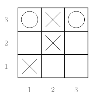
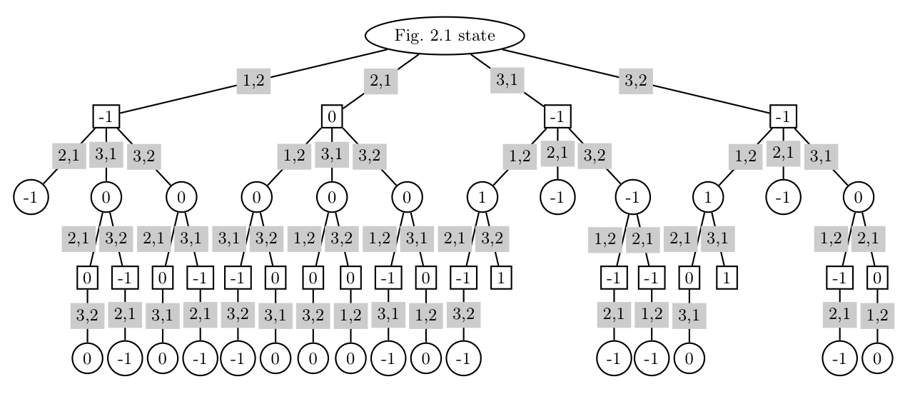
 terminal
  grow
grow 

 select
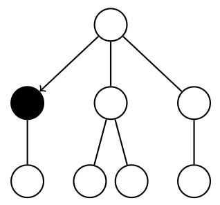
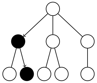
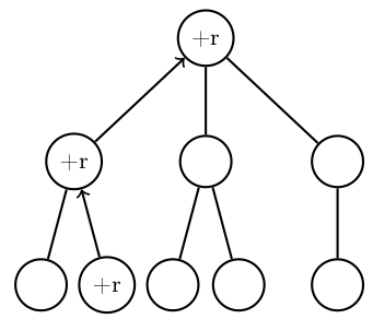
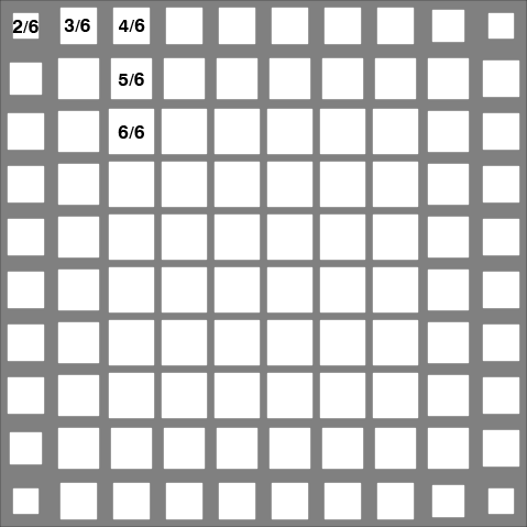
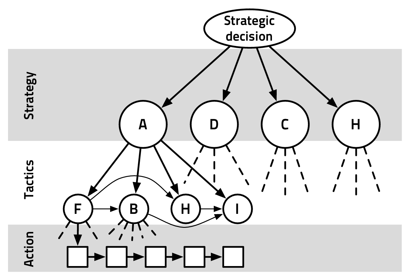
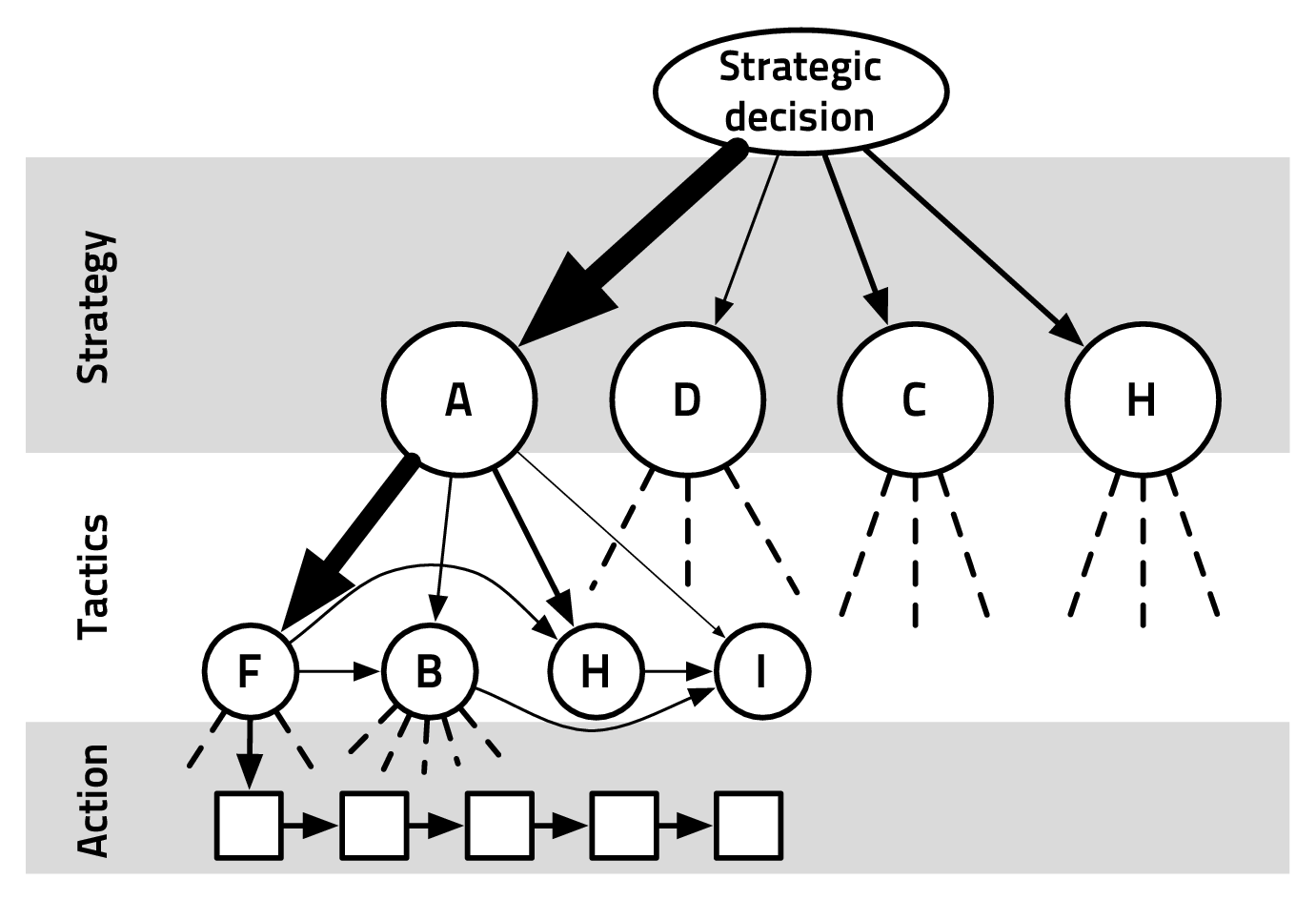
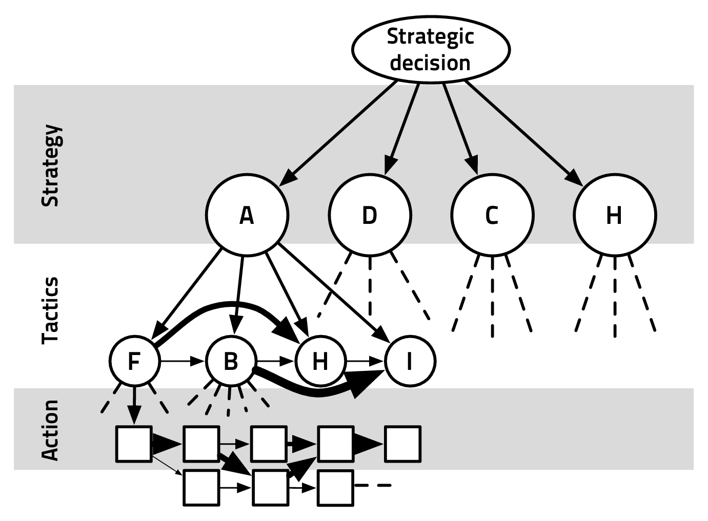
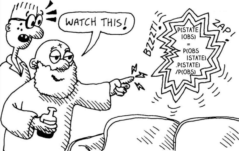
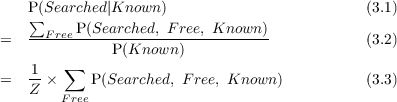
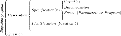
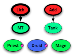
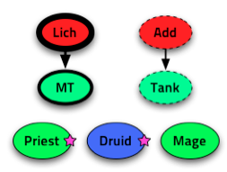
![P (S,T t- 1,t,HP1:n,D1:n,A1:n,ΔHP1:n, ID1:n,C1:n,R1:n) = (3.5)
∏n [
P(S).P (T t|Tt-1).P (T t-1). P (HPi |Ai,Ci,S,T ).P(Di|Ai,S,T).P (Ai|S,T)(3.6)
i=1 ]
P (ΔHPi |Ai,S,T).P(Ri|Ci,S,T ).P(Ci|Ai,S,T )P (IDi |T )(3.7)](phdthesis30x.png)
![(| (| (| Variables
|||| |||| |||| S,Tt-1,t,HP ,D ,A ,ΔHP ,ID ,C ,R
|||| |||| |||| 1:n 1:n 1:n 1:n 1:n 1:n 1:n
|||| |||| |||| Decomposition
|||| |||| ||{ P(S,Tt-1,t,HP1:n,D1:n,A∏1:n,[ΔHP1:n,ID1:n,C1:n,R1:n) =
|||| |||| Spec.(π) P(S)P(T|Tt-1)P (T t- 1) ni=1 P(HPi |Ai,Ci,S,T)P(Di|Ai,S,T)
|||| |{ |||| P(Ai|S,T )P (ΔHPi |Ai,S,T )P (Ri|Ci,S,T)P(Ci|Ai,S,T )P(IDi|T )]
||{ Desc.| |||| Forms
BP |||| ||||
|||| |||| |||( probability tables parametrized on wether i is targeted
|||| ||||
|||| |||| Identification (using δ)
|||| |||| learning (e.g.Laplace succession law) or manually specified
|||| |(
||||
|||( Question
P(S,T|Tt-1,HP1:n,D1:n,A1:n,ΔHP1:n,ID1:n,C1:n,R1:n)](phdthesis37x.png)
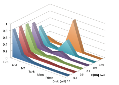
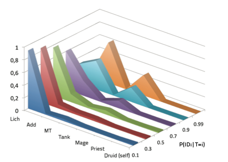
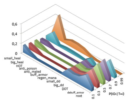
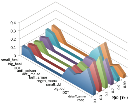
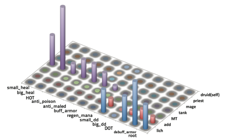
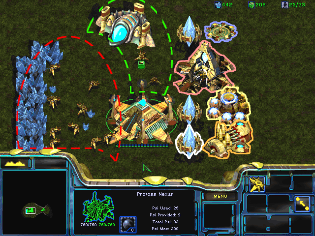
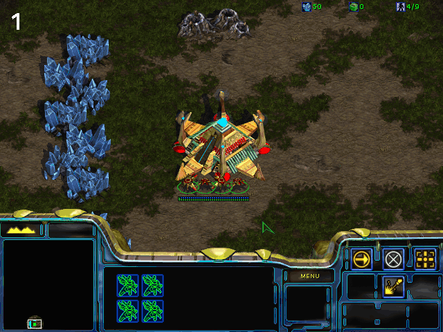
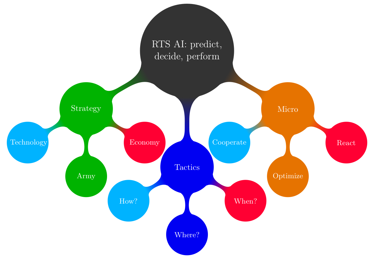
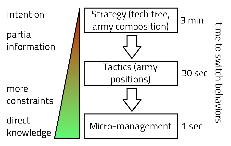
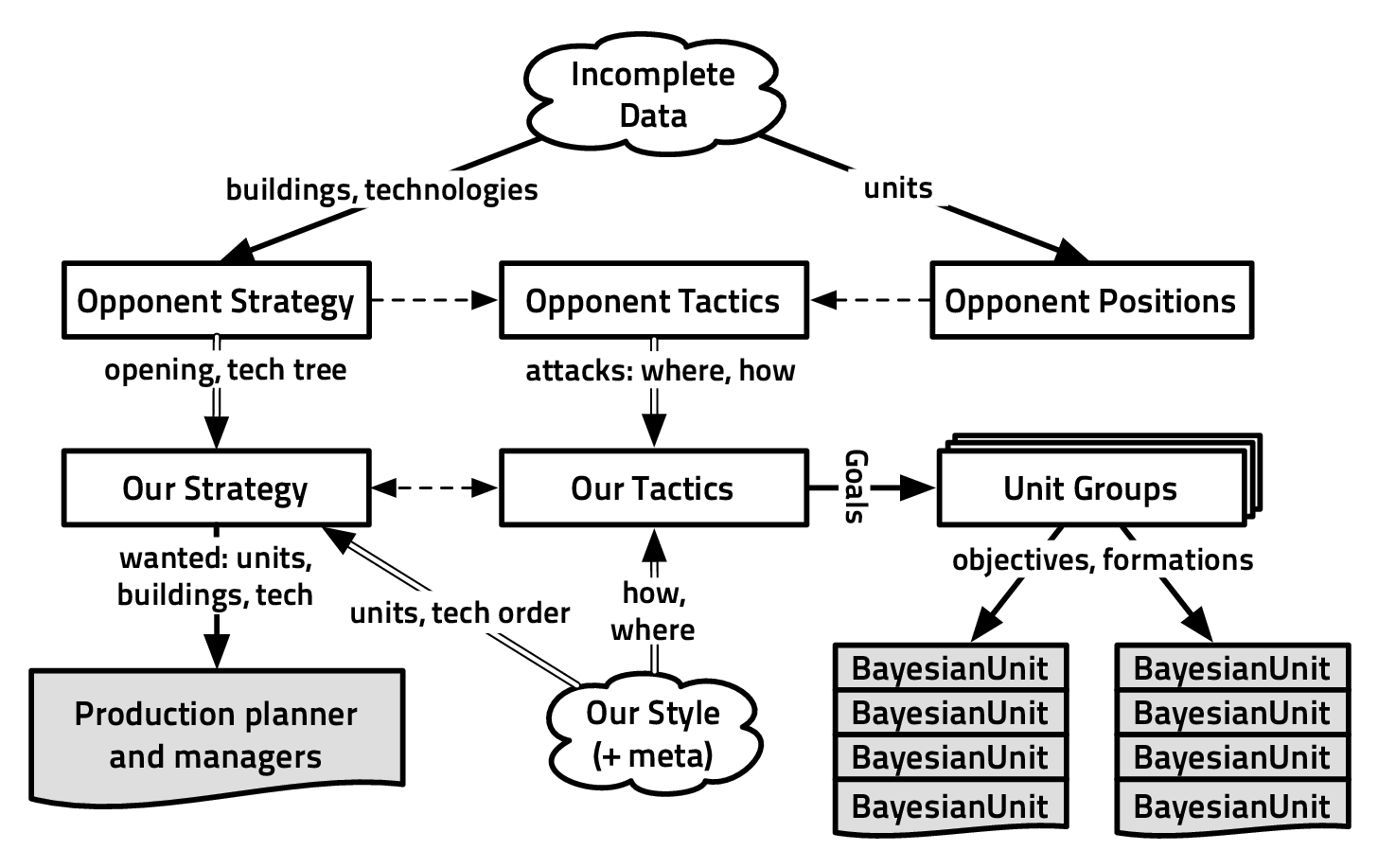
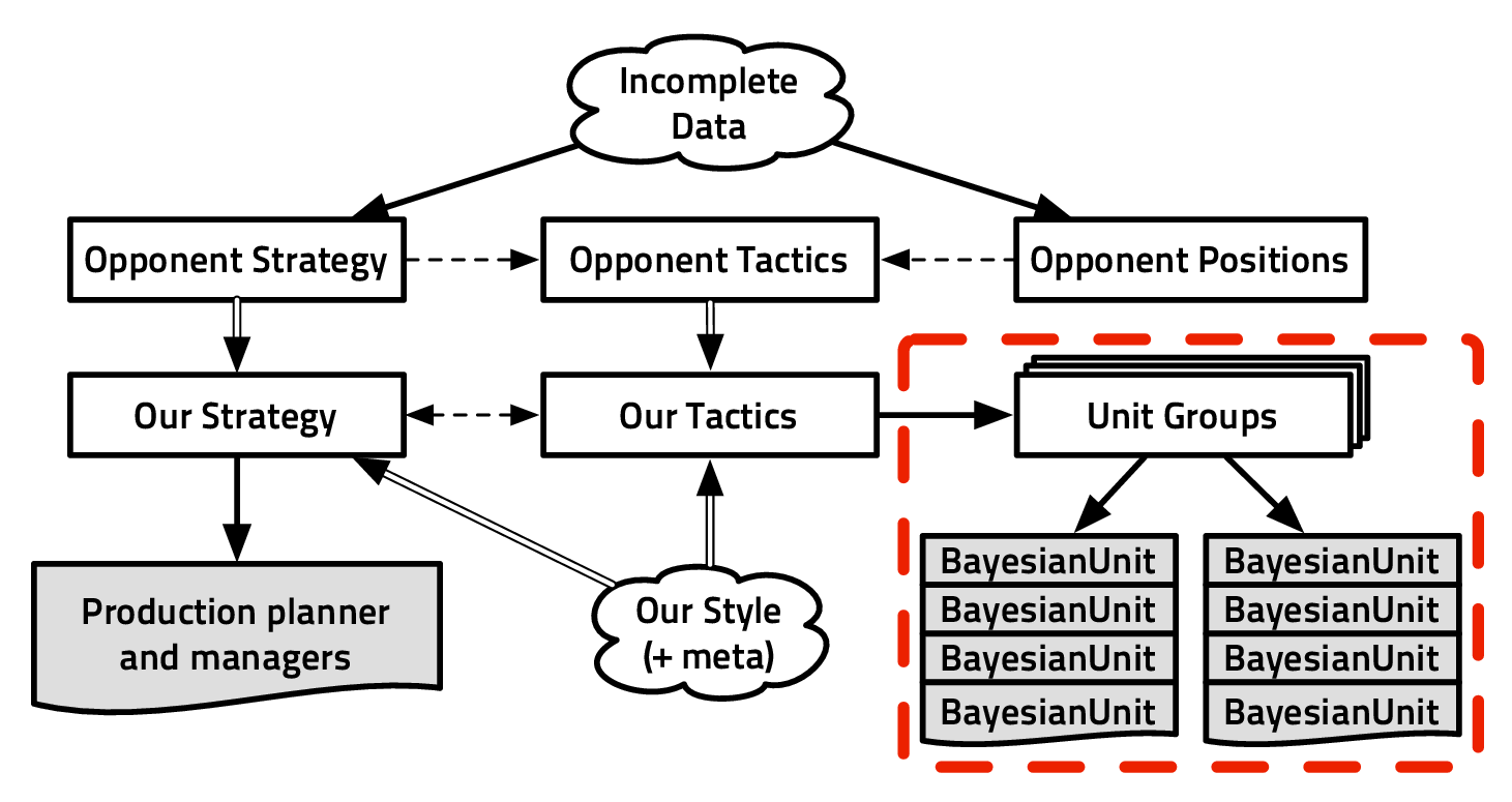
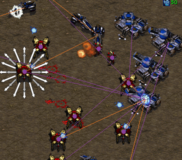

 ) are represented for a unit
with white and grey arrows around it. Orange lines represent units’ targets,
purple lines represent units’ priority targets (which are objective directions in
) are represented for a unit
with white and grey arrows around it. Orange lines represent units’ targets,
purple lines represent units’ priority targets (which are objective directions in
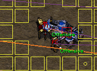
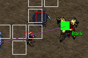
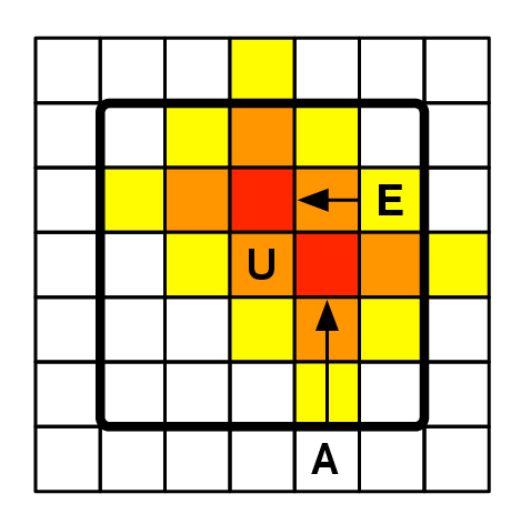
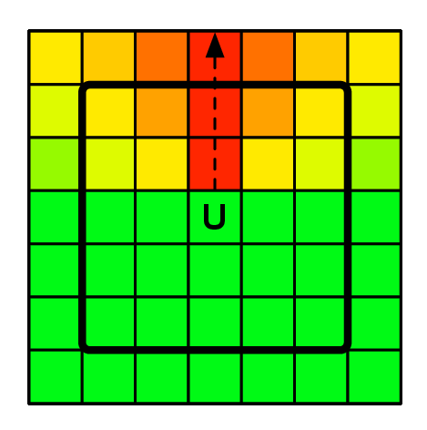
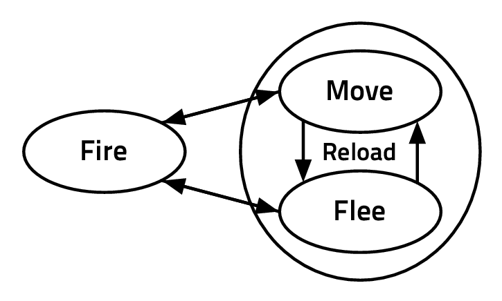
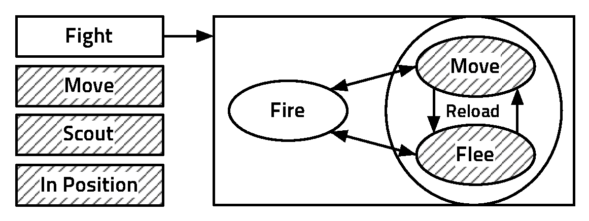
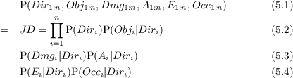
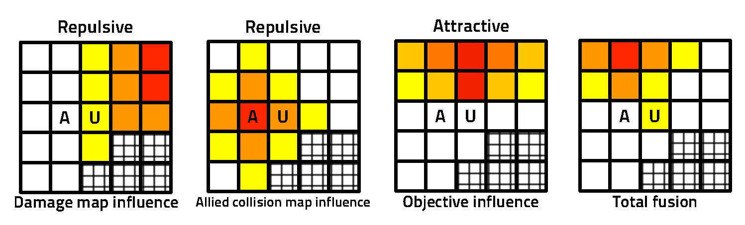
![( ( (
||| ||| ||| V ariables
|||| |||| |||| Dir1:n,Obj1:n,Dmg1:n, A1:n,E1:n,Occ1:n
|||| |||| |||| Decomposition
|||| |||| |||| ∏n [
|||| |||| { P(Dir1:n,Obj1:n,Dmg1:n,A1:n,E1:n,Occ1:n) = i=1 P(Diri)]
||||Sp|{ecifica||tioPn(O(bπj)i|Diri)P(Dmgi |Diri)P(Ai|Diri)P(Ei|Diri)P(Occi|Diri)
De||||scri|ption|||| F orms
{ |||| |||| P(Diri) : prior on directions (crossing policy)
Bayesian p||rog||||ram |||| P(XY Zi|Diri) : probability tables
|||| |||| |(
|||| ||||
|||| |||( Identification (using δ)
|||| reinforcement learning or hand specified (or distribs. parameters optimization)
||||Question
||||fightmoving∕fleeing∕scouting : P(Dir1:n|Obj1:n,Dmg1:n,A1:n,E1:n,Occ1:n)
|(](phdthesis63x.png)
![( ( (
||| || ||| V ariables
|||| |||| |||| Dir1:n,Obj1:n,Att1:n,A1:n,E1:n,Occ1:n
|||| |||| |||| Decomposition
|||| |||| |||| ∏n [
|||| |||| { P(Dir1:n,Obj1:n,Att1:n,A1:n,E1:n,Occ1:n) = i=1 P(Diri) ]
||||Sp||||ecifica||tioPn(O(bπj)i|Diri)P(Ai|Diri)P(Ei|Diri)P(Occi|Diri)P(Atti|Diri)
De||||scri{ption|||| F orms
|||| || |||| P(Diri) : prior on directions (crossing policy)
|{ |||| |||| P(XY Zi|Diri) : probability tables
Bayesian p|rog||||ram |(
|||| ||||
|||| |||| Identification
|||| |||| learning or hand specified
|||| (
||||Question
||||
||||without flocking (no Att1:n variables) : P(Dir1:n|Obj1:n,A1:n,E1:n,Occ1:n)
|||(with flocking : P(Dir1:n|Obj1:n,A1:n,E1:n,Occ1:n,Att1:n)](phdthesis70x.png)
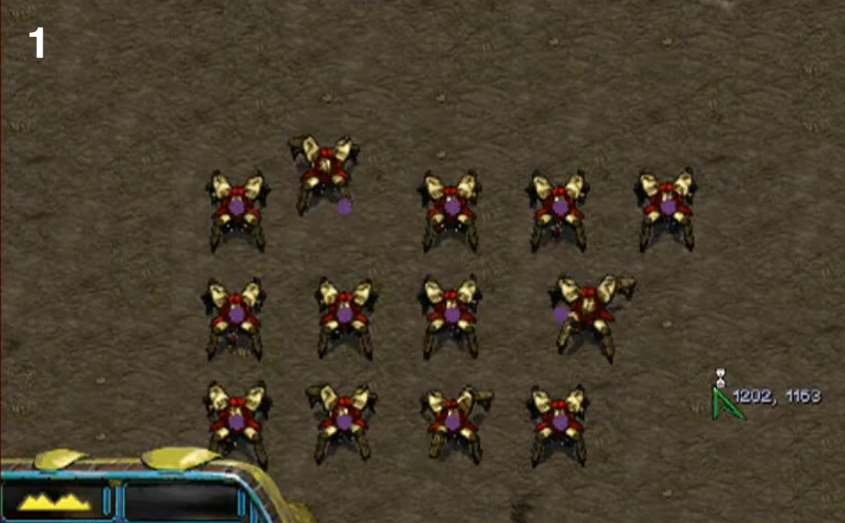
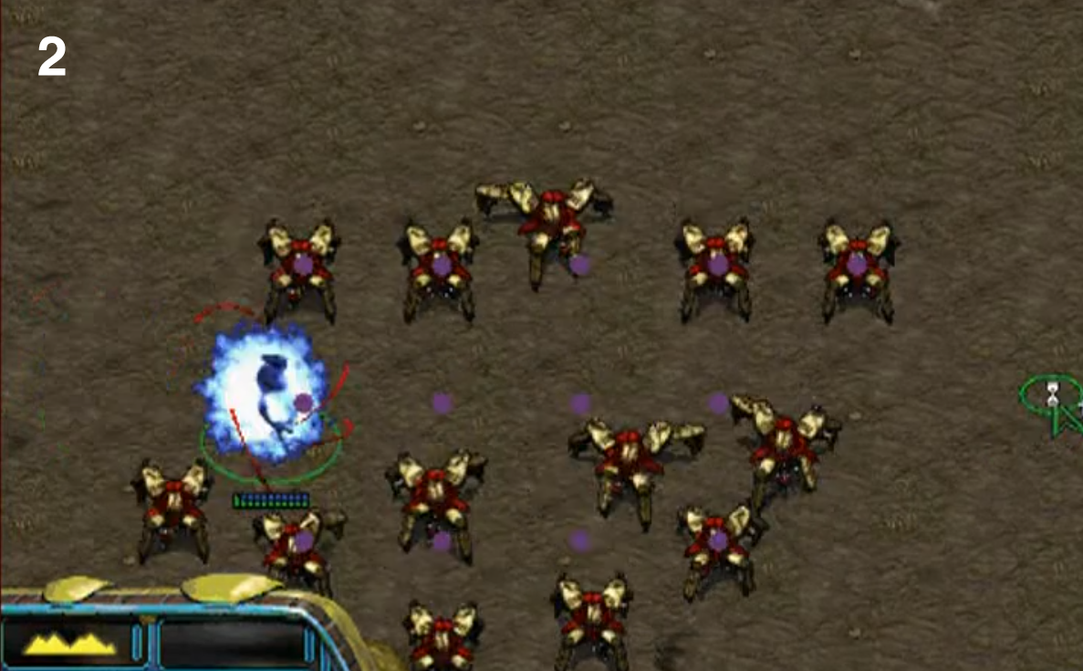
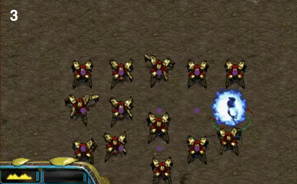
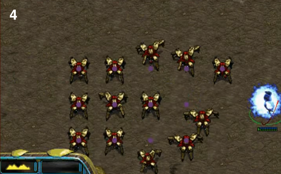
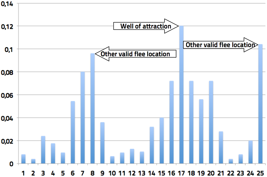
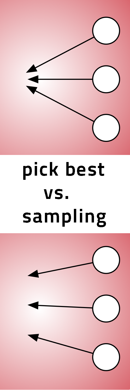
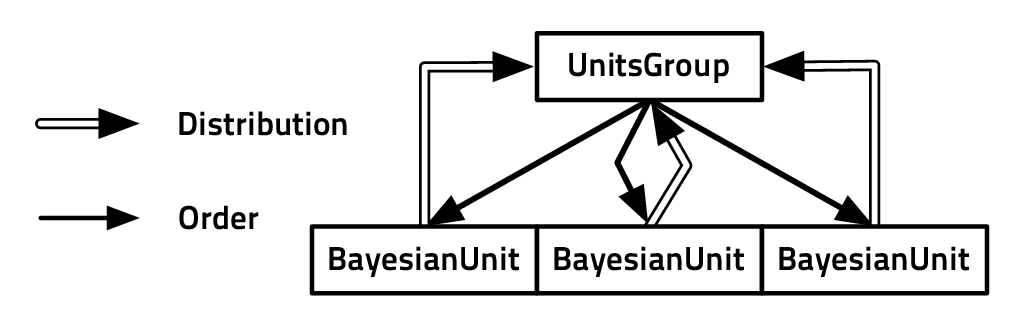
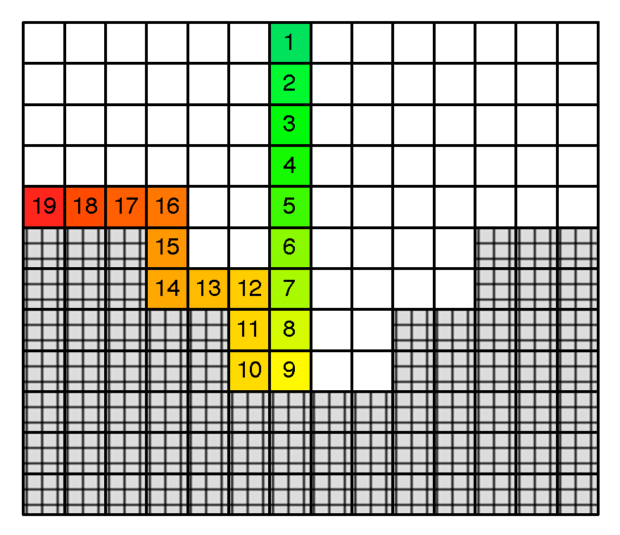
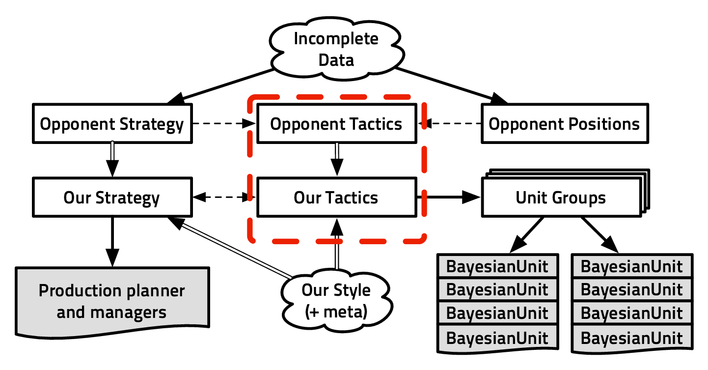
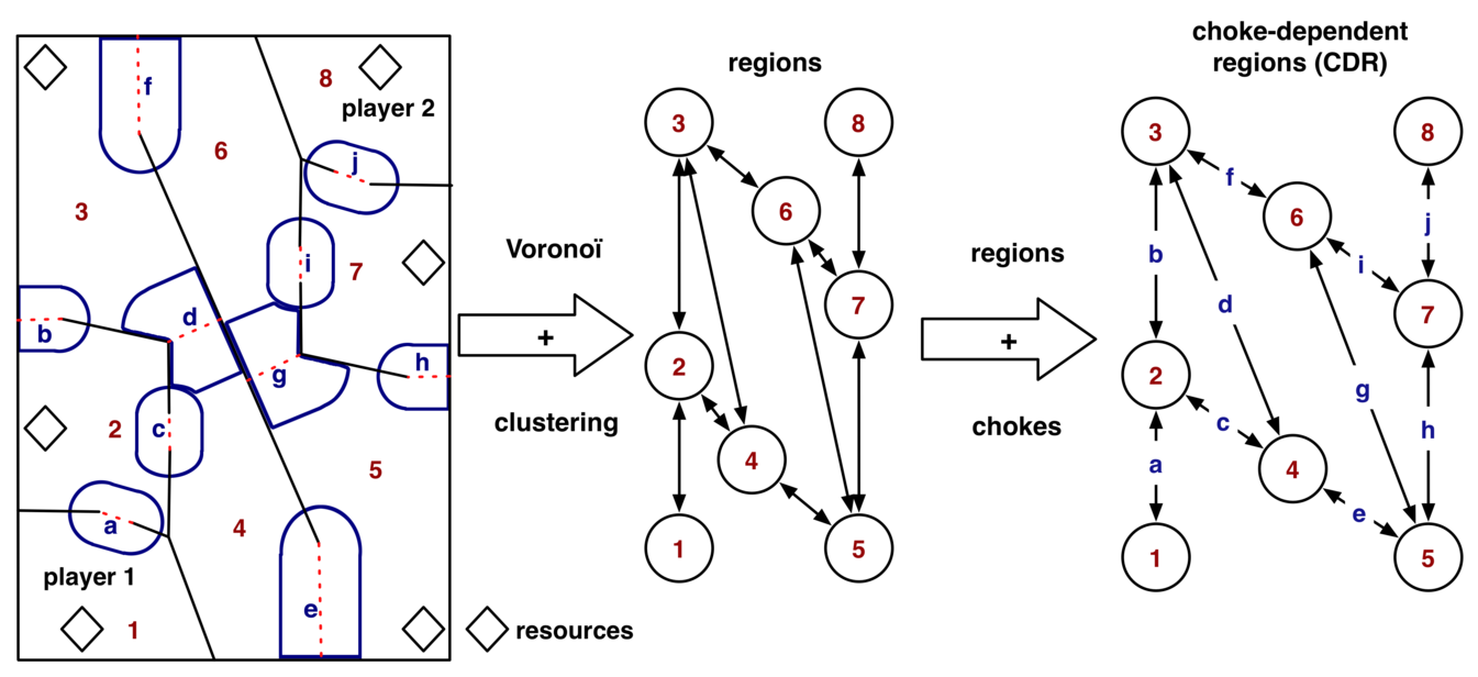
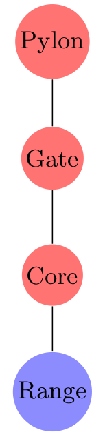
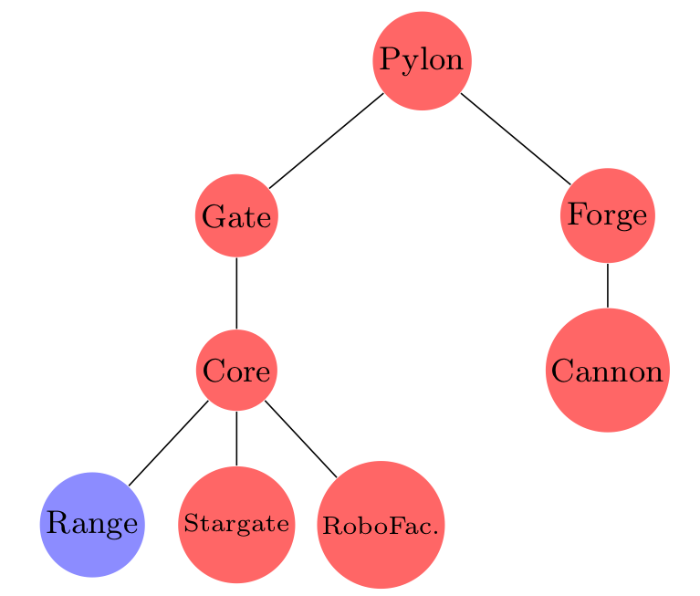

 new attack constructor
 takes units ranges into account
 ![P(A1:n,E1:n,T1:n,T A1:n,B1:n, (6.1)
H1:n,GD1:n,AD1:n,ID1:n,HP,T T) (6.2)
∏n
= [P (Ai)P (Ei,Ti,TAi,Bi|Ai) (6.3)
i=1
P (ADi, GDi,IDi |Hi)P(Hi|HP )]P(HP |T T)P(TT ) (6.4)](phdthesis83x.png)
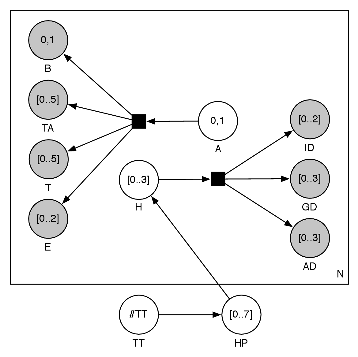
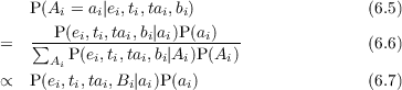
![P(∑Hi = hi|adi,gdi,idi) (6.8)
∝ [P(adi,gdi,idi|hi)P (hi|HP )P(HP |T T)P(TT )] (6.9)
TT,HP](phdthesis88x.png)
![( ( (
||| ||| ||| V ariables
|||| |||| |||| A1:n,E1:n,T1:n,T A1:n,B1:n,H1:n,GD1:n,AD1:n, ID1:n,HP, TT
|||| |||| |||| Decomposition
|||| |||| ||||
|||| |||| |||| P(A∏1n:n,E1:n,T1:n,T A1:n,B1:n,H1:n,GD1:n,AD1:n, ID1:n,HP, TT )
|||| |||| |||| = i=1 [P (Ai)P(Ei,Ti,TAi,Bi|Ai)
|||| |||| |||| P (ADi, GDi,IDi |Hi)P(Hi|HP )]P(HP |T T)P(TT )
|||| |||| { F orms
||||Sp||||ecifica||tioPn(A(iπ))prior on attack in region i
|||| |||| ||||
|||| |||| |||| P(E,T, TA,B |A ) covariance∕probability table
|||| |||| |||| P(AD, GD, ID |H ) covariance∕probability table
|||| |{ |||| P(H |HP ) = Categorical(4,HP )
De||||scri|ption|||| P(HP = hp|T T) = 1.0 iff T T → hp, else P (HP |TT ) = 0.0
|||| |||| |||| P(TT ) comes from a strategic model
|{ |||| |(
Bayesian p|rog||||ram
|||| |||| Identification (using δ) μ
|||| |||| P(A = true) = nbattlens+bantntloest battles =-bμraettgileosn∕gs∕ammaep (probability to attack a region)
|||| |||| it could be learned online (preference of the opponent) :
|||| |||| P(A = true) = --∑-1+nbattles(i)---- (online for each game ∀r)
|||| |||| i 2+ j∈regionsnbattles(i) 1+n (e,t,ta,b)
|||| |||| P(E = e,T = t,T A = ta,B = b|A = True) = |E|×|T|×|T-A|×|B|+-ba∑tEtl,esT,TA,B-nbattles(E,T,TA,B-)
|||| |||| P(AD = ad,GD = gd,ID = id|H = h) =------------1+nb∑attles(ad,gd,id,h)-----------
|||| |||| ---1+nbattles(h,hp)-|AD|×|GD |×|ID|+ AD,GD,IDnbattles(AD,GD,ID,h)
|||| |||( P(H = h |HP = hp) = |H|+∑H nbattles(H,hp)
||||
||||Questions
||||∀i ∈ regionsP(A |e,t,ta)
|||| i i i i
||||∀i ∈ regionsP(Hi|adi,gdi,idi)
|||(P (A,H |F ullyObserved)](phdthesis90x.png)
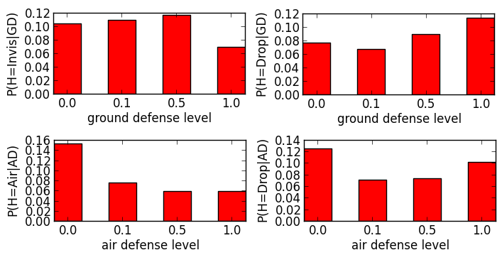

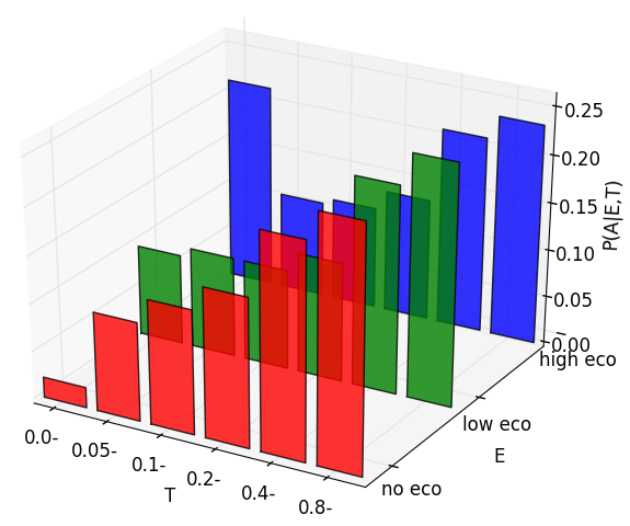


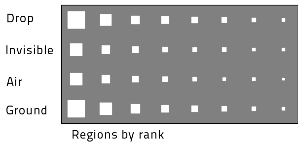
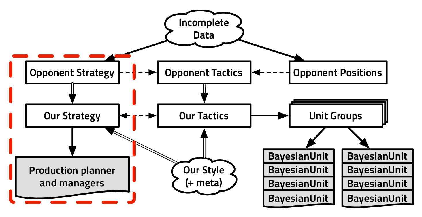
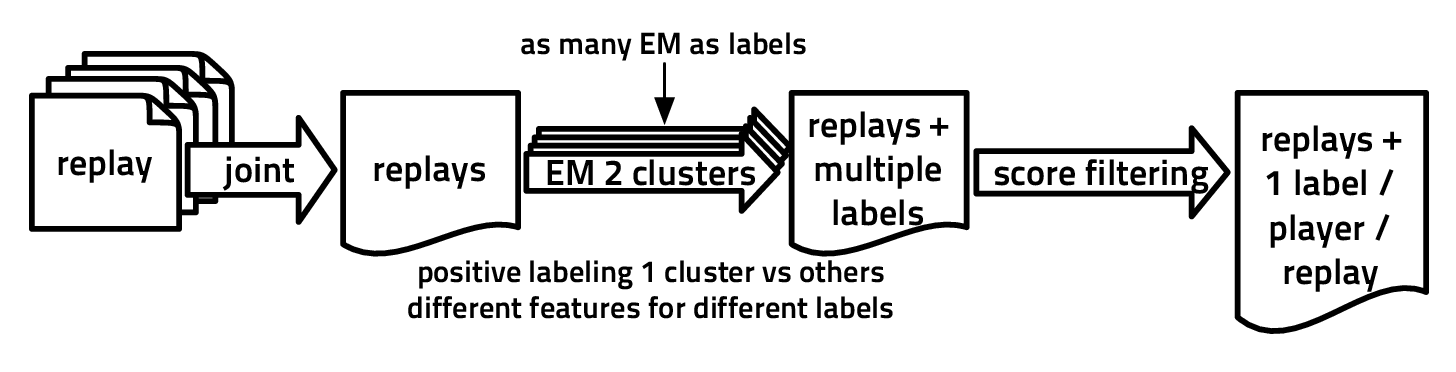
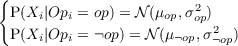
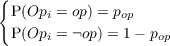
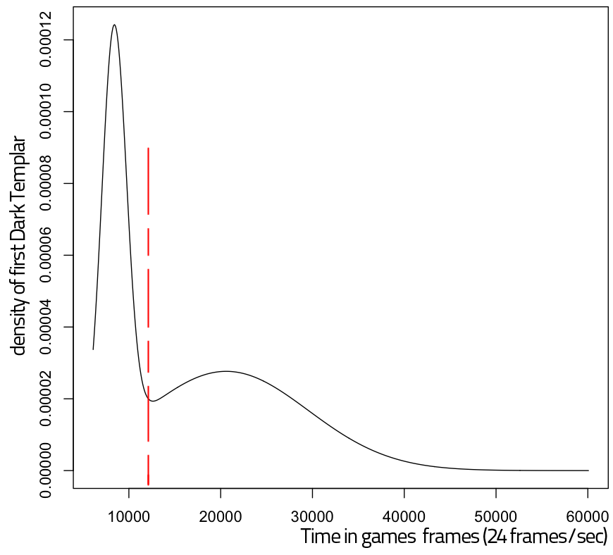
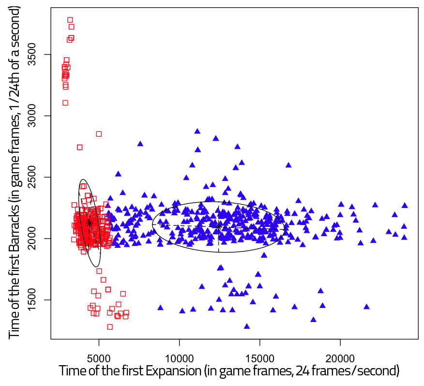
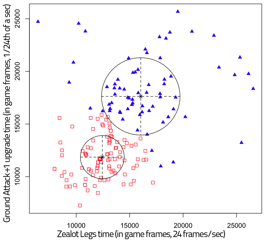
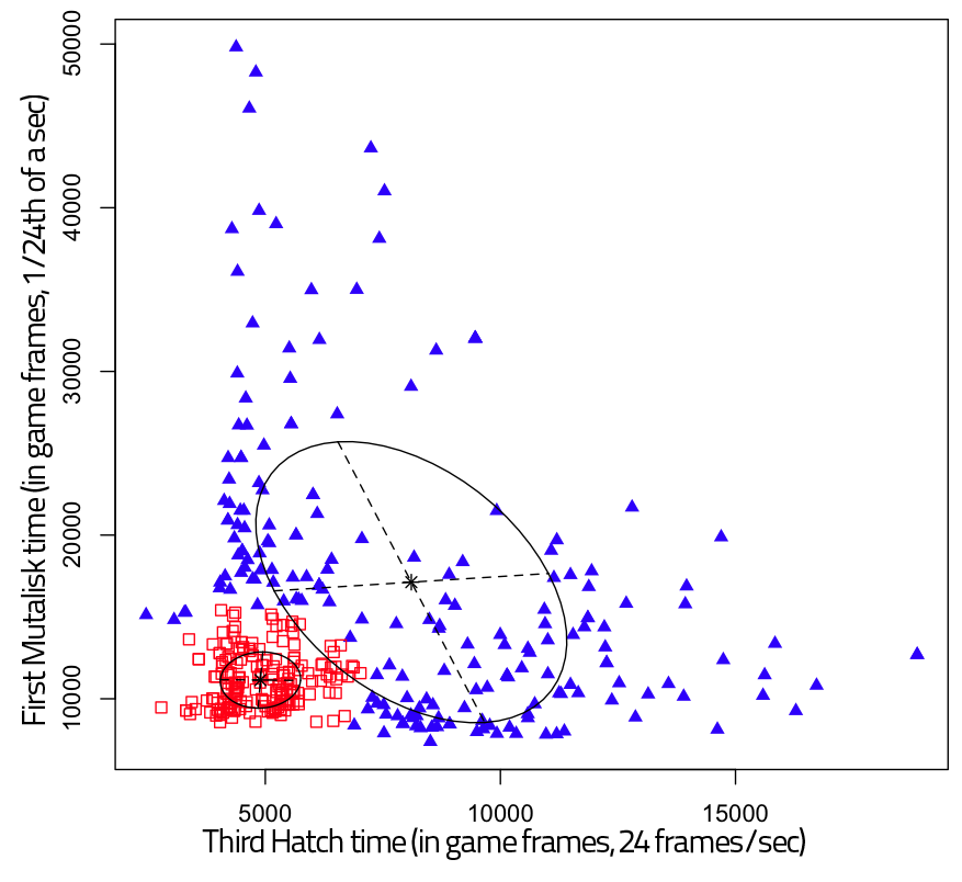
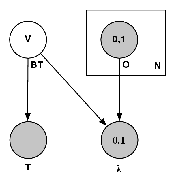
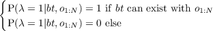
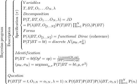
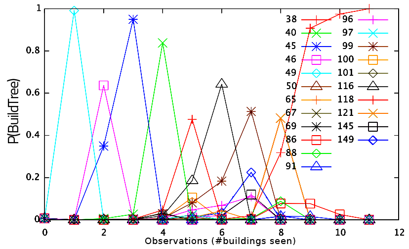
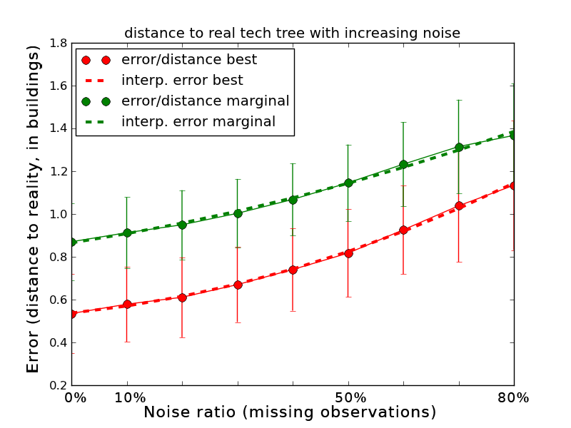
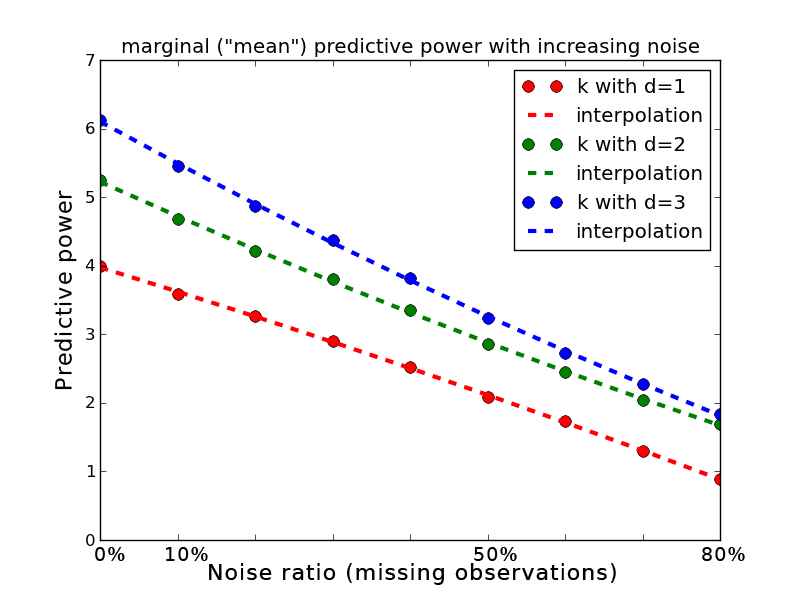
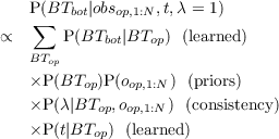
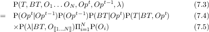
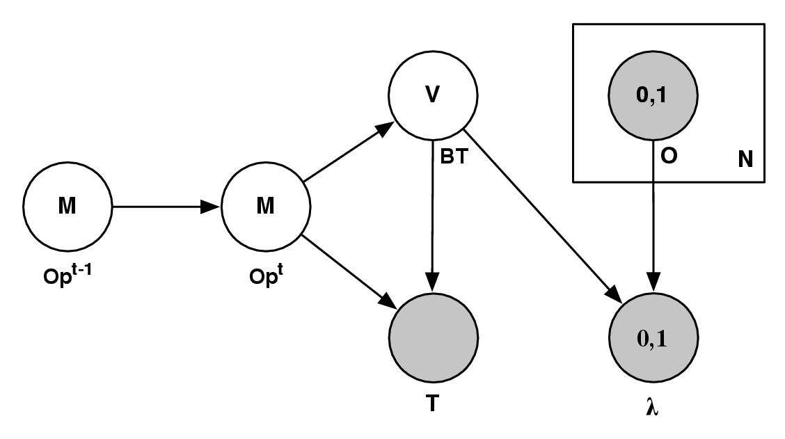
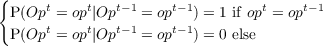

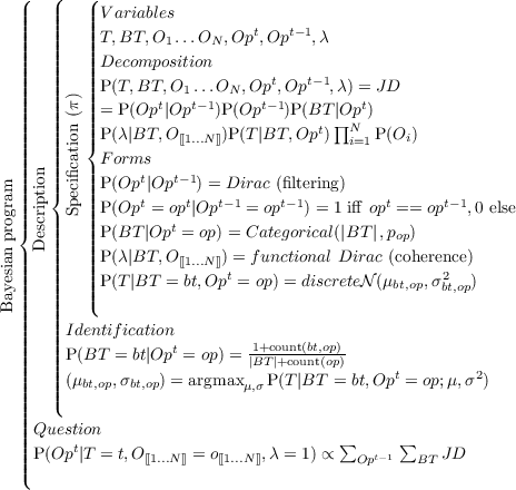
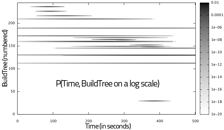
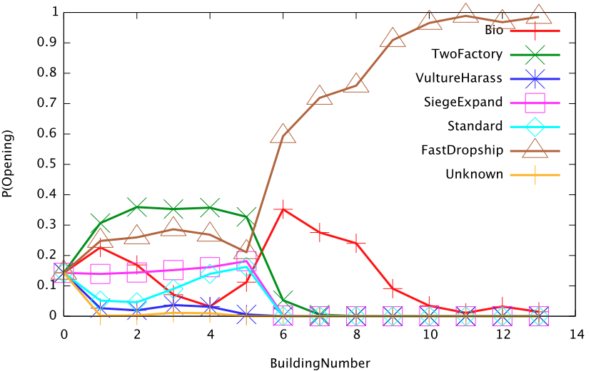
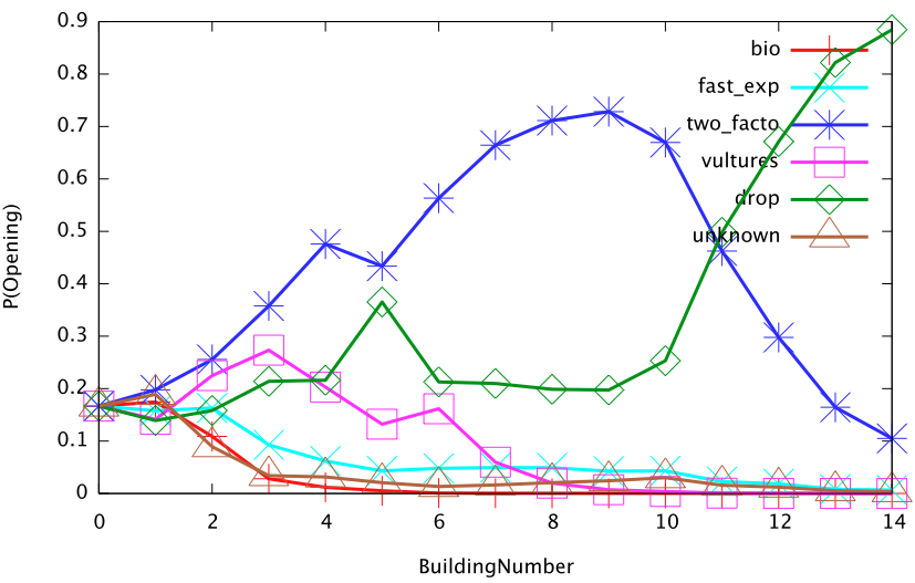
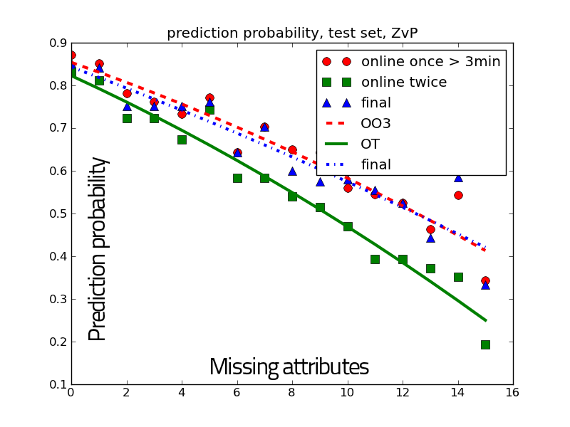
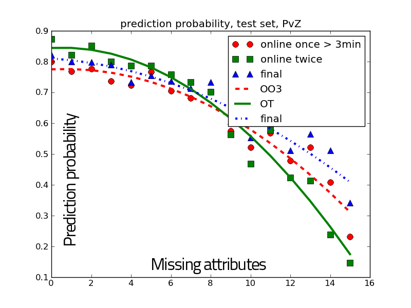
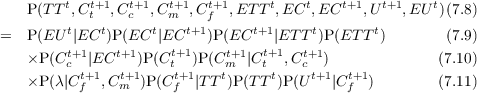
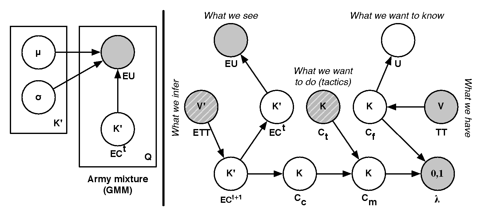
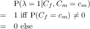
![P(U t+1|eut,ttt,λ = 1) (7.12)
∑ [ t+1 t t
∝ t t t+1 P(EC |ET T )P(ET T ) (7.13)
ETT ,EC ,EC ∑ [
×P (eut|ECt) P(Ctc+1|ECt+1 ) (7.14)
Ct+f1,Ctm+1,Ctc+1,Ctt+1
t+1 t+1 t t+1 t+1 t+1 t+1 ]]
×P (Ct )P (C f |tt)P(λ|Cf ,C m )P (U |Cf ) (7.15)](phdthesis128x.png)
![( ( (
||| ||| || V ariables
|||| |||| |||| TT t,Ct+t1,Ct+c1,Ct+m1,Ct+f1,ET Tt,ECt,ECt+1, Ut+1,EU t
|||| |||| |||| Decomposition
|||| |||| |||| t t+1 t+1 t+1 t+1 t t t+1 t+1 t
|||| |||| |||| P(TT ,Ctt ,Ct c ,C mt ,Ctf+1,ET Tt,+E1C ,ECt ,U t,EU )
|||| |||| |||| = P(EU |EC )P(EC |EC )P (EC |ETT )P (ET T )
|||| |||| |||| ×P (Ctc+1|ECt+1 )P(Ctt+1)P (Ct+m1 |Ctt+1,Ctc+1)
|||| |||| |||| ×P (λ|Ct+f1,Ct+m1)P(Ctf+1|TTt)P(TT t)P(U t+1|Ctf+1)
|||| |||| |||| F orms
|||| |||| |||| t t 2
|||| |||| |{ P(EU t|EC t+=1 ec) =t+N1(μec,σec) ′
||||Sp||||ecifica|tioPn(E(Cπ)|EC = ec ) = Categorical(K ,pect+1)
|||| |||| |||| P(ECt+1 |ET T t = ett) = Categorical(K ′,pett)
|||| |||| |||| P(ET Tt) = Categorical(V ′,pett), comes from an other model
|||| ||{ |||| P(Ct+1|ECt+1 = ec) = Categorical(K,pec)
De||||scription|||| ct+1
|||| |||| |||| P(Ctt+1) =tC+a1tegto+r1ical(K, ptat+c1) t+1
|||| |||| |||| P(Cm |Ct ,Cc ) = αP (C t ) +(1 - α)P (Cc )
||{ |||| |||| P(λ = 1|Cf ,Cm = cm) = 1 iff P (Cf = cm ) ⁄= 0, else 0
Bayesian prog||||ram |||| P(Ctf+1 = cf|TT = tt) = 1 iff cf producible with tt, else 0
|||| |||| |||| P(U t+1|Ct+1= c) = N (μc,σ2)
|||| |||| ||( f c
|||| ||||
|||| |||| Identification
|||| |||| μc,σc learned by EM on the full dataset
|||| |||| μec,σec learned by EM on the full dataset
|||| |||| P(ECt = ect|ECt+1 = ect+1) = 1+P(ect)P-(ect+1)×count(ect→ect+1)
|||| |||| t+1 t 1+P(ecK)×+cPo(uenctt(+e1c∧)×ectot)unt(ect+1)
|||| |||| P(EC = ec|ETT = ett) = K′+count(ett)
|||| |||| P(Ct+c1 = c|ECt+1 = ec) = 1+PK(c+)PP(e(ec)c×)ccoouunnttbbatattltleses((cec>)ec)
|||| |(
||||Question
|||| t+1 t t
||||P (∑U |eu ,tt ,λ = 1[)
||||∝ ET Tt,ECt,ECt+1 P (ECt+1 |ETT t)P (ET T t)
||||×P (eut|ECt )∑ t+1 t+1 t+1 t+1[P (Ct+1|ECt+1 )
|||| Cf ,Cm ,Cc ,Ct c ]]
||||×P (Ctt+1)P(Ctf+1|ttt)P (λ|Ctf+1,Ctm+1)P(Ut+1|Ct+f1 )
|(](phdthesis131x.png)
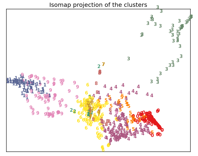
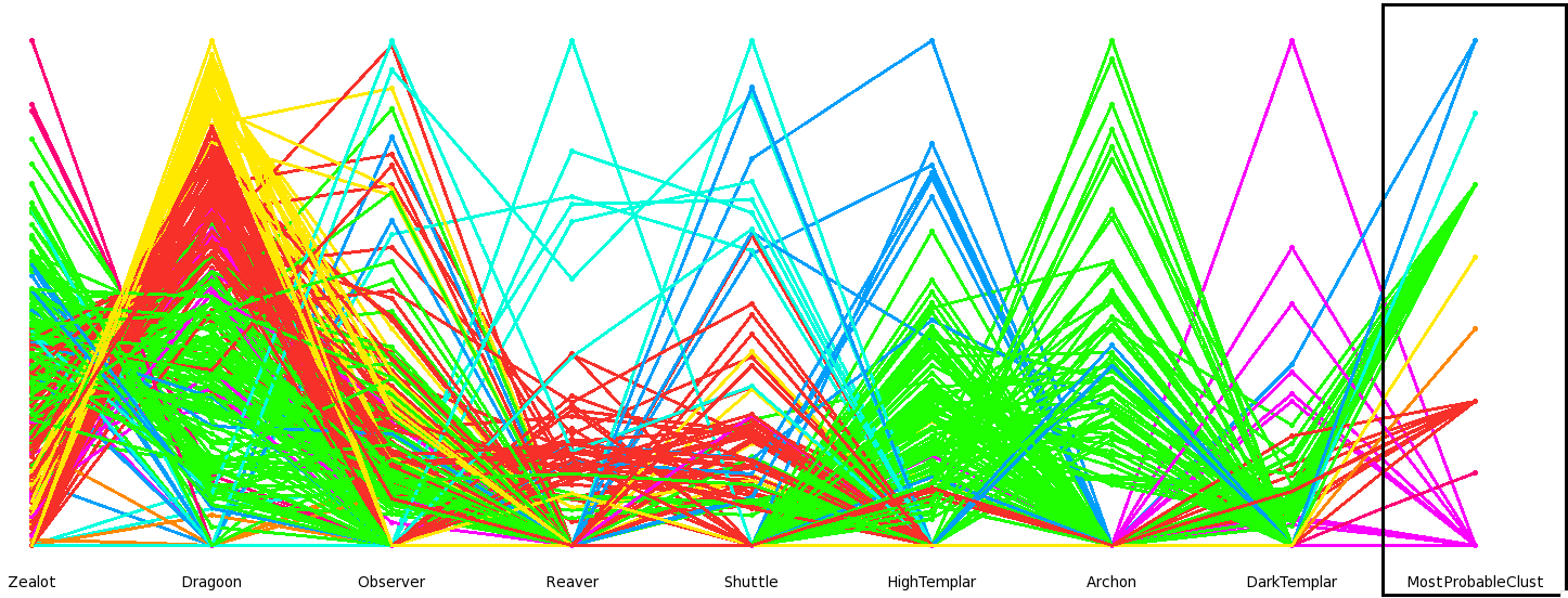
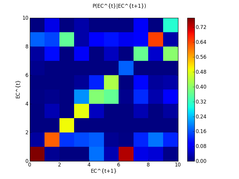
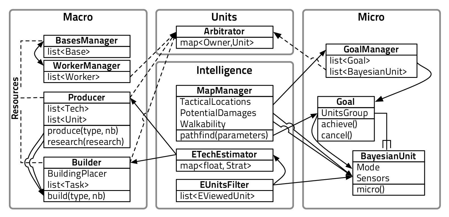
![P(Agg,U T1:m,Xt1-:m1,,t1:n) (8.1)
∏n [ ]
= P(Agg) P(U Ti)P(Xt-i 1)P(Xti|Xt-i 1,U Ti,Agg ) (8.2)
i=1](phdthesis132x.png)
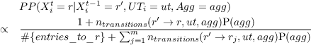
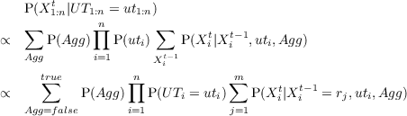
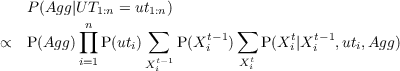
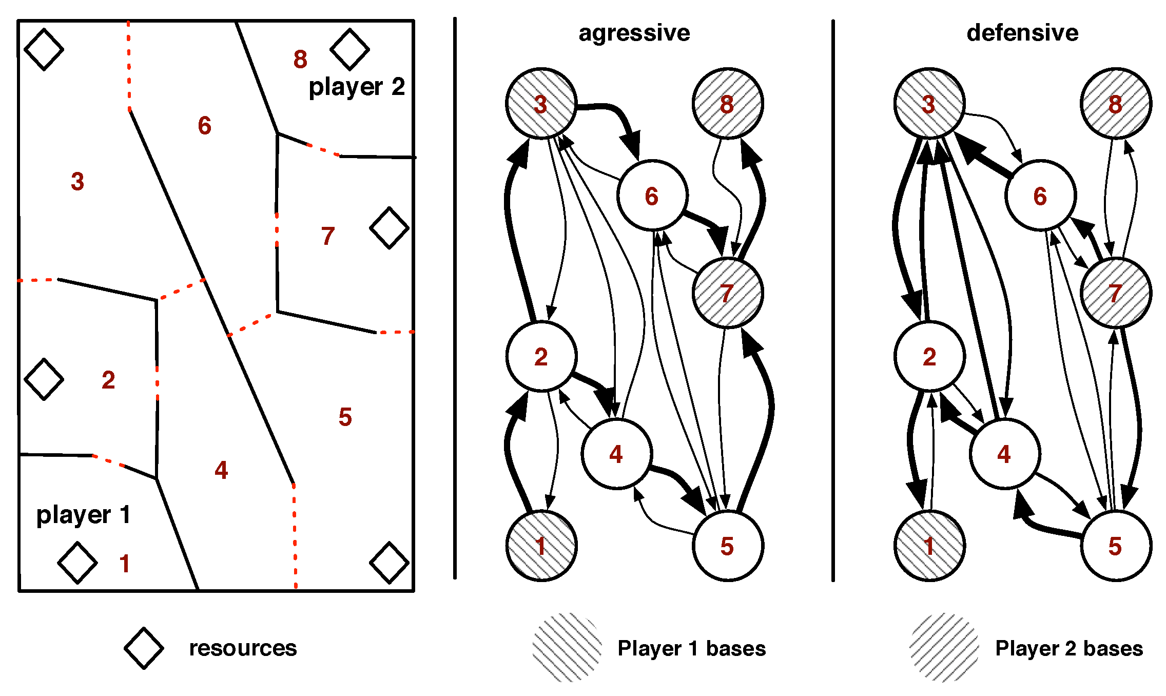
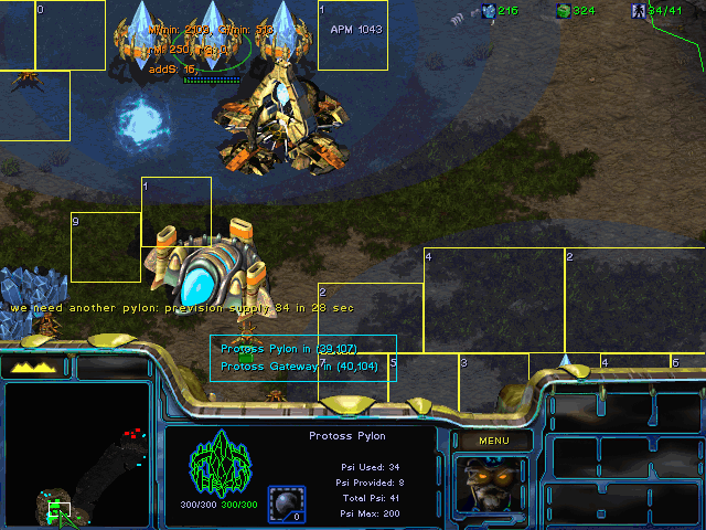
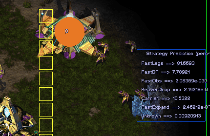
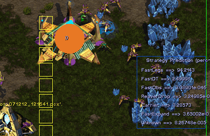
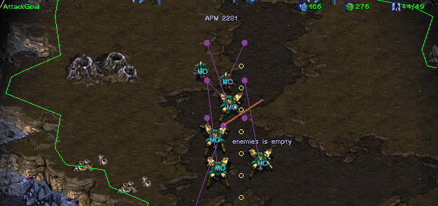
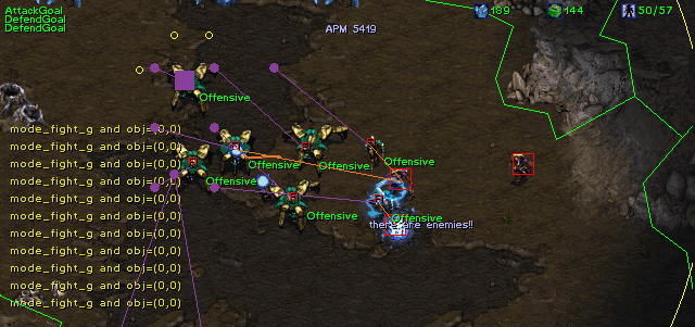
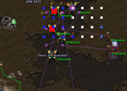
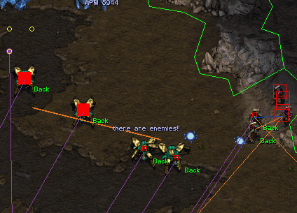
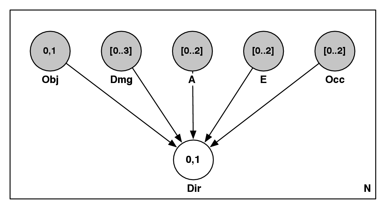


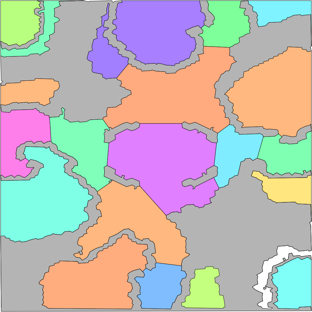
![P(A1:n,E1:n,T1:n,TA1:n,B1:n,B′1:n,λB,1:n,T′1:n,λT,1:n, (B.1)
E′1:n,λE,1:n,ID ′1:n,λID,1:n,GD ′1:n,λGD,1:n,AD ′1:n,λAD,1:n, (B.2)
H1n:n,GD1:n,AD1:n,ID1:n,HP, T T) (B.3)
= ∏ [P (A )P(E ,T ,TA ,B |A ) (B.4)
i=1 i i i i i i
P(λ |B ,B ′ )P(B′ )P (λ |T ,T ′ )P (T ′ ) (B.5)
B,i 1:n 1′:n 1′:n T,i 1:n 1:n ′ 1:n ′
P(λE,i|E1:n,E 1:n)P(E1:n)P(λID,i|ID1:n,ID1:n)P(ID 1:n) (B.6)
P(λGD,i|GD1:n,GD ′1:n)P (GD ′1:n)P (λAD,i|AD1:n,AD ′1:n)P(AD ′1:n()B.7)
P(ADi, GDi,IDi|Hi)P(Hi|HP )]P (HP |T T)P(TT ) (B.8)](phdthesis155x.png)
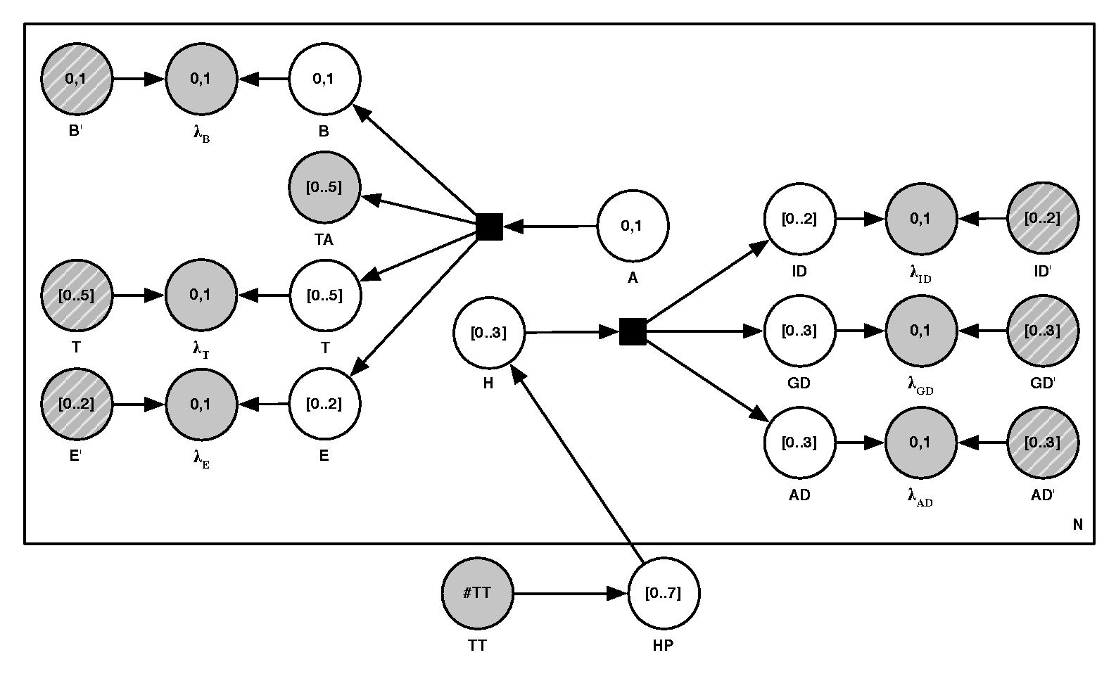
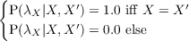
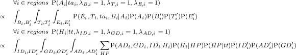
![( ( (
|||| |||| ||||Variables ′ ′ ′
||||| ||||| |||||A1:n′,E1:n,T1:n,TA1′:n,B1:n,B1:n,λ′B,1:n,T1:n,λT,1:n,E1:n,λE,1:n,
||||| ||||| |||||ID1:n,λID,1:n,GD 1:n,λGD,1:n,AD1:n,λAD,1:n,H1:n,GD1:n,AD1:n,ID1:n,HP, TT
||||| ||||| |||||Decomposition ′ ′ ′
||||| ||||| |||||P(A′1:n,E1:n,T1:n,T′A1:n,B1:n,B1:n′,λB,1:n,T1:n,λT,1:n,E1:n,λE,1:n,
||||| ||||| |||||I=D1∏:nn,λI[PD(,1A:n,)GPD(E 1:,nT,λ,GTDA,1,:nB,A|AD1):Pn,(λλAD,|B1:n,H,B1:n′,G)PD(1B:n′,A)DP1(:λn,ID|T1:n,,HTP′,)PT(TT)′ )
||||| ||||| |||||P(λi=1|E1:ni,E ′ i)P(Ei′ )iP(λi i|ID1:nB,,iID1′:n)P1(I:Dn′ )P1(:nλ |T,GiD11:n:n,GD1:n′ )P(1G:nD ′ )
||||| ||||| ||{P(λEA,iD,i|AD1:1n:,nAD′ 1):nP(ADI′D,)iP (ADi,GD1i:n,IDi|Hi1:)nP(Hi|GHDP,i)]P(HP|TT)1:Pn(TT) 1:n
|||||Spe|||||cificatio||nF (oπr)ms 1:n 1:n
||||| ||||| |||||P(Ar) prior on attack in region i
||||| ||||| |||||P(E,T,TA,B|A ) covariance∕probability table
||||| ||||| |||||P(λX|X, X′)=1.0 iff X = X′, else P(λX|X,X ′)= 0.0 (Dirac)
De|||||scrip{tion|||||P(AD,GD,ID |H ) covariance∕probability table
||||| |||| |||||P(H|HP)= Categorical(4,HP)
||{ ||||| |||||P(HP = hp|TT)= 1.0 iff TT → hp, else P(HP |TT)= 0.0
Bayesianpr||ogra|||||m ||||(P(TT) comes from a strategic model
||||| |||||
||||| ||||| Identification (using δn) μbattles∕game
||||| ||||| P(Ar = true)= nbattlesb+atntlneots battles = μregions∕map (probability to attack a region)
||||| ||||| it could be learned online (preference of the opponent):
||||| ||||| P(Ar = true)= 2+-∑i1+∈nrebgaiottnlessnb(ra)ttles(i) (online for each game)
||||| ||||| P(E = e,T = t,TA = ta,B =b|A = True)=-----------1+nba∑ttles(e,t,ta,b)-----------
||||| ||||| --|E|×|T|×|TA1|×+|n∑Bb|+attlesE(,aT,d,TgdA,,Bid,hn)battles(E,T,TA,B)
||||| ||||| P(AD =ad,GD =gd,ID =id|H = h)= |AD|×|GD |×|ID|+ AD,GD,ID nbattles(AD,GD,ID,h)
||||| ||||| P(H = h|HP =hp)= |H|+1+∑nHbanttbleas(tthle,hsp(H),hp)
||||| (
||||| Questions
||||| decision - making
||||| ∀i∈regionsP(Ai|tai,λB,i = 1,λT,i =1,λE,i = 1)
||||( ∀i∈regionsP(Hi|tt,λID,i = 1,λGD,i = 1,λAD,i =1)](phdthesis158x.png)