![[*]](crossref.png) ), that is, it is not necessarely
normalized.
), that is, it is not necessarely
normalized.
The prevoius definition restricts
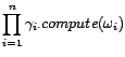 |
A joint distribution is provided of the method
![]() returning:
returning:
 |
(3.20) |
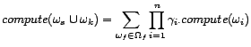
where
![]() (i.e.
(i.e. ![]() is the complement of
is the complement of
![]() on
on
![]() ) and
) and ![]() is the projections of
is the projections of
![]() on
on ![]() .
.